The Bloch Sphere

The Bloch sphere is perhaps the most intuitive way in which to understand basic single qubit gates, as we can interpret them as rotations between different states. In this short blog, we will use it to build an intuition for the single qubit gates x, y, z, h, s, rx, ry, rz, and how statevectors and bases works.

 

​x






#We first import numpy and matplotlib as they have useful functions.
 
 
import numpy as np
 
from math import pi
 
import matplotlib.pyplot as plt
 
%matplotlib inline
 

 
#When then import everything from qiskit, and more specifically the
 
#function for plotting a statevector in a bloch sphere.
 
import qiskit as qk
 
from qiskit.visualization import plot_bloch_vector
 
# make the imports that are necessary for our work
 
from qiskit import ClassicalRegister, QuantumRegister, QuantumCircuit
 
from qiskit import execute, Aer
 
from qiskit import IBMQ
 
from qiskit.visualization import plot_histogram
 

 
# We import the qasm_simulator which simulates the noise one would
 
# see while using NISQ devices.
 
backend = Aer.get_backend('qasm_simulator')
 
 
 
 
 
 

The shots variable determines the amount of samples we use to negate some of the random noise that is simulated. Setting this lower may lead to more prevalent noise, while higher values will require more computing time.

xxxxxxxxxx
 
 
 
 
 
 
shots = 10000 #Try to set me to 1, 10, 100, 1000, 10 000 and run the circuit below!
 
 
 
 
 
 

The three variables below define three different basis. For now, we will leave them as they are and return to them a bit later in this notebook.

xxxxxxxxxx
 
 
 
 
 
 
 
# Z measurement of qubit 0
 
 
measure_z = QuantumCircuit(1,1)
 
measure_z.measure(0,0)
 

 
# X measurement of qubit 0
 
measure_x = QuantumCircuit(1,1)
 
measure_x.h(0)
 
measure_x.measure(0,0)
 

 
# Y measurement of qubit 0
 
measure_y = QuantumCircuit(1,1)
 
measure_y.sdg(0)
 
measure_y.h(0)
 
measure_y.measure(0,0);
 
 
 
 
 
 

With our bases in place, we can now define our function for simulating a circuit and returning a statevector.

xxxxxxxxxx
 
 
 
 
 
 
 
# Our function takes the single qubit quantum circuit 'qc'
 
 
def simulate_circuit(qc):
 
    bloch_vector = [] #We create a list to store the information for each basis.
 
    for measure_circuit in [measure_x, measure_y, measure_z]: #We measure for each basis
 

 
        # Run the circuit with a the selected measurement and get the number of samples that output each bit value
 
        # We execute our circuit, add the transformation into the basis we care about (measure_circuit), 
 
        # use the QASM backeck, and sample equal to the amount of 'shots'.
 
        counts = execute(qc+measure_circuit, backend,shots=shots).result().get_counts()
 
        # We then calculate the probabilities for each bit value
 
        probs = {}
 
        for output in ['0','1']:
 
            if output in counts:
 
                probs[output] = counts[output]/shots
 
            else:
 
                probs[output] = 0
 
        bloch_vector.append( probs['0'] -  probs['1'] )
 
    #We then return the bloch vector containing probabilities for each basis.
 
    return bloch_vector
 
 
 
 
 
 

You don't need to be able to replicate the code above, but know that it samples measurements from each basis by running the circuit several times (to get reliable results, upwards of 1000 to 10000 shots are not uncommon).

Now it is time to feed the function some circuits and see how the gates transforms the statevector of the qubit!

First, here are some gates to play around with:

Method	Description
.x(0)	Flips state around x-axis
.y(0)	Flips state around y-axis
.z(0)	Flips state around z-axis
.h(0)	Switches z and x values by flipping around axis between $|0⟩$$\vert0\rangle$ and x
.s(0)	Switches x and y values
.rx($\theta$$\theta$,0)	Rotate $\theta$$\theta$ radians around the x-axis.
.ry($\theta$$\theta$,0)	Rotate $\theta$$\theta$ radians around the y-axis.
.rz($\theta$$\theta$,0)	Rotate $\theta$$\theta$ radians around the z-axis.

Note that the 0's just specifies which qubit to apply the gate to. This will be useful for later multiqubit circuits!

xxxxxxxxxx
 
 
 
 
 
 
 
# We create a quantum circuit with just 1 qubit.
 
 
qc = QuantumCircuit(1)
 

 
# PUT GATES YOU WISH TO APPLY HERE!
 
#qc.h(0)
 
qc.ry(pi/2,0)
 
# We send the circuit to our simulator
 
result = simulate_circuit(qc)
 

 
# And plot the resulting statevector on a bloch sphere
 
plot_bloch_vector(result)
 
 
 
 
 
 

 

 

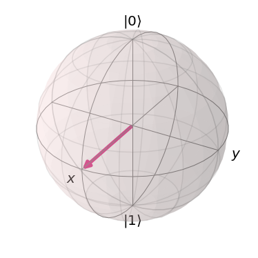
Task 1: Apply each gate individually and see what it does. (Hint: If nothing happens, the gate rotates around an axis with which you are currently parallel to. Use another gate to no longer be parallel.)

Question 1: Is .ry(pi/2, 0) equivalent to the Hadamard gate,.h(0)? Why, why not?
Question 2: Does the order of the gates matter to the final position of the statevector? Question 3: Identify the axis around which the phase gate, .s(0), rotates.

Challenge 1: Construct a circuit that ends at negative x (opposite of where a single Hadamard would leave you).
Challenge 2: Construct a circuit which goes through all the poles of the x, y, and z, axes.
Challenge 3: Construct a circuit that gives equal probability of measuring 0 and 1, and x and -x if you measured a single time.
Challenge 4: Construct a circuit which gives 75% chance of measuring 1 and 25% of measuring 0 in the z basis.

Choosing a Basis

Remember how we skipped over how we measure the different bases? Let's look at it again. Unless otherwise specified, qubits are always initialized to $|0⟩$$\vert0\rangle$, which means the qubit has a 100% chance (disregarding noise) to be measured as a 0 in the Z basis, something often called the computational basis. One can think of a basis as simply seeing how far along one of the axes the statevector is. When we measure in Qiskit, we measure the computational basis. However, this gives us no information about the x and y components of the statevector.

Challenge: Can you figure out how the bases that we've copied from above gives us information about the x and y components?

Hint: See them as quantum circuits, and send them to our simulator.

xxxxxxxxxx
 
 
 
 
 
 
 
# Z measurement of qubit 0
 
 
measure_z = QuantumCircuit(1,1)
 
measure_z.measure(0,0);
 

 
# X measurement of qubit 0
 
measure_x = QuantumCircuit(1,1)
 
measure_x.h(0)
 
measure_x.measure(0,0)
 

 
# Y measurement of qubit 0
 
measure_y = QuantumCircuit(1,1)
 
measure_y.sdg(0)
 
measure_y.h(0)
 
measure_y.measure(0,0);
 
 
 
 
 
 

Final notes about bases: Unlike normal bits that can be either 0 or 1, the different superpositions between amplitude and phase that are intrinsic to qubits leaves us with a lot of freedom when it comes to measuring their value. While we've only mentioned the x, y, and z basis, one could imagine an infinite amount of axes within the sphere, all of which are valid bases. However, as the quantum state of qubits collaps once we measure them, we must choose our basis with care, since we only get one measurement for every time we run the circuit. That is why we set shots to such a large number above, so that we can average over many measurements, and the reason we ran a for-loop which meant we ran these many repetition for each basis. This is what allowed us to obtain all components of our statevector above.

Entanglement

Quantum entanglement is a physical phenomenon that occurs when pairs or groups of particles are generated or interact in ways such that the quantum state of each particle cannot be described independently instead, a quantum state must be described for the system as a whole. This means for an entangled system, the quantum state of composite system cannot be factored as a product of states of its local constituents.

Therefore, it can only be expressed as a sum, or superposition, of products of states of local constituents with more than one term, i.e., a state $|\psi ⟩$$|\psi\rangle$ is said to be entangled if $|\psi ⟩\ne |a⟩\otimes |b⟩$$|\psi\rangle \neq |a\rangle \otimes |b\rangle$ for any two subsystem states $|a⟩$$|a\rangle$ and $|b⟩$$|b\rangle$.

Preparing Entangled States

We will try to prepare some of the most important (and popular) entangled quantum states, and also the their applications:

1. Bell states
2. Greenberger-Horne-Zeilinger state i.e. (GHZ state)
3. W state

Bell States

The Bell states (or EPR states) are specific quantum states of two qubits that represent the simplest (and maximal) examples of quantum entanglement.

 

$|{\mathrm{\Phi }}^{\pm }⟩=\frac{|00⟩\pm |11⟩}{\sqrt{2}}$$|\Phi^{\pm}\rangle = \frac{|00\rangle \pm |11\rangle}{\sqrt{2}}$ $|{\mathrm{\Psi }}^{\pm }⟩=\frac{|01⟩\pm |10⟩}{\sqrt{2}}$$|\Psi^{\pm}\rangle = \frac{|01\rangle \pm |10\rangle}{\sqrt{2}}$

Preparing Bell States

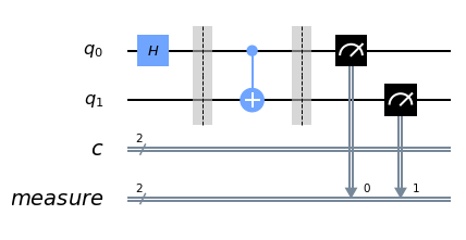
In quantum circuit language, the way to create a Bell pair between two qubits is to first transfer one of them to the Bell basis ($|+⟩$$|+\rangle$ and $|-⟩$$|-\rangle$) by using a Hadamard gate, and then to apply a CNOT gate onto the other qubit controlled by the one in the Bell basis.

Implementation

xxxxxxxxxx
 
 
 
 
 
 
 
qc = QuantumCircuit(2, 2)
 
 
qc.h(0) #rotates Z to X and vice-versa
 
qc.barrier()
 
qc.cx(0, 1) 
 
qc.measure_all() #performs measurement on all qubits
 
qc.draw(output='mpl')
 
 
 
 
 
 

 

 

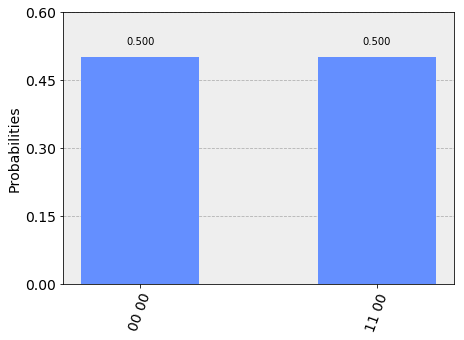
xxxxxxxxxx
 
 
 
 
 
 
 
backend = Aer.get_backend('qasm_simulator')
 
 
job_sim = execute(qc, backend, shots=1024)
 
sim_result = job_sim.result()
 

 
measurement_result = sim_result.get_counts(qc)
 
print(measurement_result)
 
plot_histogram(measurement_result)
 
 
 
 
 
 

xxxxxxxxxx
 
 
 
 
 
 
{'00 00': 512, '11 00': 512}
 
 
 
 
 
 

 

 

 

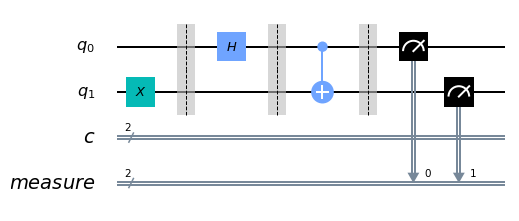
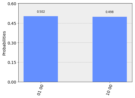
xxxxxxxxxx
 
 
 
 
 
 
 
qc = QuantumCircuit(2, 2)
 
 
qc.x(1) #Flipping the initial state of the qubit
 
qc.barrier()
 
qc.h(0)
 
qc.barrier()
 
qc.cx(0, 1)
 
qc.measure_all()
 
qc.draw(output='mpl')
 
 
 
 
 
 

 

 

xxxxxxxxxx
 
 
 
 
 
 
 
backend = Aer.get_backend('qasm_simulator')
 
 
job_sim = execute(qc, backend, shots=1024)
 
sim_result = job_sim.result()
 

 
measurement_result = sim_result.get_counts(qc)
 
print(measurement_result)
 
plot_histogram(measurement_result)
 
 
 
 
 
 

xxxxxxxxxx
 
 
 
 
 
 
{'01 00': 514, '10 00': 510}
 
 
 
 
 
 

 

 

 

Quantum Teleportation

The concept

Alice wants to send quantum information to Bob. Specifically, suppose she wants to send the state $|\psi ⟩=\alpha |0⟩+\beta |1⟩$$\vert\psi\rangle = \alpha\vert0\rangle + \beta\vert1\rangle$ to Bob. This entails passing on information about $\alpha$$\alpha$ and $\beta$$\beta$ to Bob.

There exists a theorem in quantum mechanics which states that you cannot simply make an exact copy of an unknown quantum state. This is known as the no-cloning theorem. As a result of this we can see that Alice can't simply generate a copy of $|\psi ⟩$$\vert\psi\rangle$ and give the copy to Bob. Copying a state is only possible with a classical computation.

However, by taking advantage of two classical bits and entanglement, Alice can transfer the state $|\psi ⟩$$\vert\psi\rangle$ to Bob. We call this teleportation as at the end Bob will have $|\psi ⟩$$\vert\psi\rangle$ and Alice won't anymore. Let's see how this works in some detail.

How does quantum teleportation work?

Step 1: Alice and Bob create an entangled pair of qubits and each one of them holds on to one of the two qubits in the pair. The pair they create is a special pair called a Bell pair that we have discussed above.

Let's say Alice owns $q_1$$q_1$ and Bob owns $q_2$$q_2$ after they part ways.

Step 2: Alice applies a CNOT gate on $q_1$$q_1$, controlled by $|\psi ⟩$$\vert\psi\rangle$ (the qubit she is trying to send Bob).

Step 3: Next, Alice applies a Hadamard gate to $|\psi ⟩$$|\psi\rangle$, and applies a measurement to both qubits that she owns - $q_1$$q_1$ and $|\psi ⟩$$\vert\psi\rangle$.

Step 4: Then, it's time for a phone call to Bob. She tells Bob the outcome of her two qubit measurement. Depending on what she says, Bob applies some gates to his qubit, $q_2$$q_2$. The gates to be applied, based on what Alice says, are as follows :

00 $\to$$\rightarrow$ Do nothing

01 $\to$$\rightarrow$ Apply $X$$X$ gate

10 $\to$$\rightarrow$ Apply $Z$$Z$ gate

11 $\to$$\rightarrow$ Apply $ZX$$ZX$ gate

Note that this transfer of information is classical.

And voila! At the end of this protocol, Alice's qubit has now teleported to Bob.

Implementation

In this notebook, we will give Alice a secret state $|\psi ⟩$$\vert\psi\rangle$. This state will be generated by applying a series of unitary gates on a qubit that is initialized to the ground state, $|0⟩$$\vert0\rangle$. Go ahead and fill in the secret unitary that will be applied to $|0⟩$$\vert0\rangle$ before passing on the qubit to Alice.

xxxxxxxxxx
 
 
 
 
 
 
secret_unitary = 'hz'
 
 
 
 
 
 

If the quantum teleportation circuit works, then at the output of the protocol discussed above will be the same state passed on to Alice. Then, we can undo the applied secret_unitary (by applying its conjugate transpose), to yield the $|0⟩$$\vert0\rangle$ that we started with.

We will then do repeated measurements of Bob's qubit to see how many times it gives 0 and how many times it gives 1.

What do we expect?

In the ideal case, and assuming our teleportation protocol works, we will always measure 0 from Bob's qubit because we started off with $|0⟩$$|0\rangle$.

In a real quantum computer, errors in the gates will cause a small fraction of the results to be 1. We'll see how it looks.

1. Simulating the teleportation protocol

xxxxxxxxxx
 
 
 
 
 
 
 
# simple function that applies a series of unitary gates from a given string
 
 
def apply_secret_unitary(secret_unitary, qubit, quantum_circuit, dagger):
 
    functionmap = {
 
                    'x':quantum_circuit.x,
 
                    'y':quantum_circuit.y,
 
                    'z':quantum_circuit.z,
 
                    'h':quantum_circuit.h,                    
 
                    't':quantum_circuit.t,                    
 
    }
 
    if dagger: functionmap['t'] = quantum_circuit.tdg
 
    
 
    if dagger:
 
        [functionmap[unitary](qubit) for unitary in secret_unitary]
 
    else:
 
        [functionmap[unitary](qubit) for unitary in secret_unitary[::-1]]
 
 
 
 
 
 

xxxxxxxxxx
 
 
 
 
 
 
 
# Create the quantum circuit with 3 qubits and 3 classical bits
 
 
qc = QuantumCircuit(3, 3)
 

 
''' Qubit ordering as follows (classical registers will just contain measured values of the corresponding qubits):
 
q[0]: qubit to be teleported (Alice's first qubit. It was given to her after the application of a secret unitary 
 
      which she doesn't know)
 
q[1]: Alice's second qubit
 
q[2]: Bob's qubit, which will be the destination for the teleportation
 
'''
 

 
# Apply the secret unitary that we are using to generate the state to teleport. You can change it to any unitary
 
apply_secret_unitary(secret_unitary, qc.qubits[0], qc, dagger = 0)
 
qc.barrier()
 
# Next, generate the entangled pair between Alice and Bob (Remember: Hadamard followed by CX generates a Bell pair)
 
qc.h(1)
 
qc.cx(1, 2)
 
qc.barrier()
 
# Next, apply the teleportation protocol. 
 
qc.cx(0, 1)
 
qc.h(0)
 
qc.measure(0, 0)
 
qc.measure(1, 1)
 
qc.cx(1, 2)
 
qc.cz(0, 2)
 
qc.barrier()
 

 
'''
 
In principle, if the teleportation protocol worked, we have q[2] = secret_unitary|0>
 
As a result, we should be able to recover q[2] = |0> by applying the reverse of secret_unitary
 
since for a unitary u, u^dagger u = I.
 
'''
 
apply_secret_unitary(secret_unitary, qc.qubits[2], qc, dagger=1)
 
qc.measure(2, 2)
 
 
 
 
 
 

 

xxxxxxxxxx
 
 
 
 
 
 
<qiskit.circuit.instructionset.InstructionSet at 0x7fb910870250>
 
 
 
 
 
 

 

It's always a good idea to draw the circuit that we have generated in code. Let's draw it below.

xxxxxxxxxx
 
 
 
 
 
 
qc.draw(output='mpl')
 
 
 
 
 
 

 

 

xxxxxxxxxx
 
 
 
 
 
 
 
backend = Aer.get_backend('qasm_simulator')
 
 
job_sim = execute(qc, backend, shots=1024)
 
sim_result = job_sim.result()
 

 
measurement_result = sim_result.get_counts(qc)
 
print(measurement_result)
 
plot_histogram(measurement_result)
 
 
 
 
 
 

xxxxxxxxxx
 
 
 
 
 
 
{'010': 246, '001': 263, '011': 257, '000': 258}
 
 
 
 
 
 

 

 

 

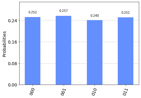
Note that the results on the x-axis in the histogram above are ordered as $c_2{c}_1{c}_0$$c_2c_1c_0$. We can see that only results where $c_2=0$$c_2 = 0$ appear, indicating that the teleporation protocol has worked.

Greenberger-Horne-Zeilinger state i.e. (GHZ state)

The Greenberger-Horne-Zeilinger state is a certain type of entangled quantum state that involves at least three subsystems (qubits). For a $N$$N$ qubit system it is defined as: $|GHZ⟩=\frac{|0{⟩}^{\otimes N}+|1{⟩}^{\otimes N}}{\sqrt{2}}$$|GHZ\rangle = \frac{|0\rangle^{\otimes N} + |1\rangle^{\otimes N}}{\sqrt{2}}$

Simply put, it is a quantum superposition of all subsystems being in state $0$$0$ with all of them being in state $1$$1$ (states $0$$0$ and $1$$1$ of a single subsystem are fully distinguishable). The GHZ state is a maximally entangled quantum state.

Here, we will try to prepare the simplest one, i.e. the 3-qubit GHZ state: $|GHZ⟩=\frac{|000⟩+|111⟩}{\sqrt{2}}$$|GHZ\rangle = \frac{|000\rangle + |111\rangle}{\sqrt{2}}$

Preparing 3-qubit GHZ state

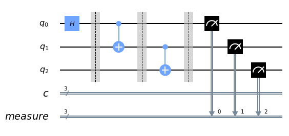
In quantum circuit language, the way to create a 3-qubit GHZ states is to first transfer the first qubit to the Hadamard basis ($|+⟩$$|+\rangle$ and $|-⟩$$|-\rangle$) by using a Hadamard gate, and then to applying two CNOT gates in pairwise fashion: ($CNOT(0,1)$$CNOT(0,1)$, $CNOT(1,2)$$CNOT(1,2)$).

Implementation

xxxxxxxxxx
 
 
 
 
 
 
 
qc = QuantumCircuit(3, 3)
 
 
qc.h(0)
 
qc.barrier()
 
qc.cx(0, 1)
 
qc.barrier()
 
qc.cx(1, 2)
 
qc.measure_all()
 
qc.draw(output='mpl')
 
 
 
 
 
 

 

 

xxxxxxxxxx
 
 
 
 
 
 
 
backend = Aer.get_backend('qasm_simulator')
 
 
job_sim = execute(qc, backend, shots=1024)
 
sim_result = job_sim.result()
 

 
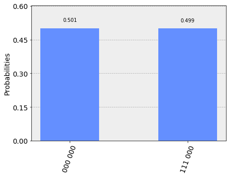
measurement_result = sim_result.get_counts(qc)
 
print(measurement_result)
 
plot_histogram(measurement_result)
 
 
 
 
 
 

xxxxxxxxxx
 
 
 
 
 
 
{'111 000': 511, '000 000': 513}
 
 
 
 
 
 

 

 

 

[#1] Challenge

Devise an algorithm to prepare the following generalized $GH{Z}_N$$GHZ_{N}$ state: $|GH{Z}_N⟩=\frac{|0{⟩}^{\otimes N}+|1{⟩}^{\otimes N}}{\sqrt{2}}$$|GHZ_{N}\rangle = \frac{|0\rangle^{\otimes N} + |1\rangle^{\otimes N}}{\sqrt{2}}$

W state

The $W$$W$ state is an entangled quantum state of three qubits which has the following shape: $W=\frac{|001⟩+|010⟩+|100⟩}{\sqrt{3}}$$W = \frac{|001\rangle + |010\rangle + |100\rangle}{\sqrt{3}}$

 

Preparing W state

We saw that construction of both Bell states and GHZ state was quite straight forward. However, preparing $W$$W$ state is quite tricky as its (one of the simplest) preparation make use of a custom gate $G(p)$$G(p)$ and anti-controlled gates.

$\begin{array}{c}G(p)=\left[\begin{array}{cc}\sqrt{1-p}& -\sqrt{p}\\ \sqrt{p}& \sqrt{1-p}\end{array}\right]\end{array}$$G(p) = \begin{bmatrix} \sqrt{1-p} & -\sqrt{p} \\ \sqrt{p} & \sqrt{1-p} \end{bmatrix}$

This can be implemented as a $U_3(\theta ,\varphi ,\lambda )$$U_{3}(\theta,\phi,\lambda)$ gate with $\varphi =\lambda =0$$\phi=\lambda=0$, which amounts to a standard SU(2) representation of a rotation of angle $\theta$$\theta$ around the y-axis.

$\begin{array}{c}{U}_3(\theta ,\varphi ,\lambda )=\left[\begin{array}{cc}\cos \frac{\theta }{2}& -e^{-\iota \lambda }\sin \frac{\theta }{2}\\ e^{\iota \varphi }\sin \frac{\theta }{2}& e^{\iota (\lambda +\varphi )}\cos \frac{\theta }{2}\end{array}\right]\end{array}$$U_{3}(\theta,\phi,\lambda) = \begin{bmatrix} \cos{\frac{\theta}{2}} & -e^{-\iota\lambda}\sin{\frac{\theta}{2}} \\ e^{\iota \phi}\sin{\frac{\theta}{2}} & e^{\iota(\lambda+\phi)}\cos{\frac{\theta}{2}} \end{bmatrix}$

Therefore, in our case for $p=1/3$$p=1/3$, we have $\theta =2\times {\cos }^{-1}\sqrt{1-p}$$\theta=2\times\cos^{-1}{\sqrt{1-p}}$. Moreover, the anti-controlled gates can be implemented $AC-U=XC-UX$$AC-U = XC-UX$, i.e. sandwiching controlled gate bebtween two $X$$X$ gates.

Implementation

xxxxxxxxxx
 
 
 
 
 
 
 
qc = QuantumCircuit(3, 3)
 
 
# Custom Gate (G(1/3))
 
qc.u3(2*np.arccos(np.sqrt(2/3)),0,0,0)
 
qc.barrier()
 
# Anti-Controlled Hadamamrd
 
qc.x(0)
 
qc.ch(0, 1)
 
qc.x(0)
 
qc.barrier()
 
# Anti-Controlled toffoli
 
qc.x(0)
 
qc.x(1)
 
qc.ccx(0, 1, 2)
 
qc.x(1)
 
qc.x(0)
 
qc.measure_all()
 
qc.draw(output='mpl')
 
 
 
 
 
 

 

 

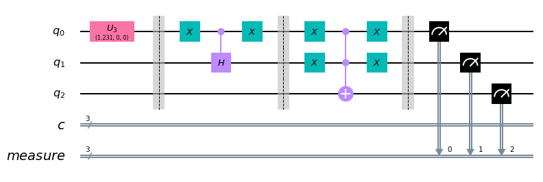
xxxxxxxxxx
 
 
 
 
 
 
 
backend = Aer.get_backend('qasm_simulator')
 
 
job_sim = execute(qc, backend, shots=2048)
 
sim_result = job_sim.result()
 

 
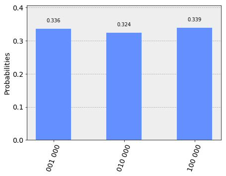
measurement_result = sim_result.get_counts(qc)
 
print(measurement_result)
 
plot_histogram(measurement_result)
 
 
 
 
 
 

xxxxxxxxxx
 
 
 
 
 
 
{'100 000': 695, '010 000': 664, '001 000': 689}
 
 
 
 
 
 

 

 

 

[#2] Challenge

Devise an algorithm to prepare the following generalized $W_N$$W_{N}$ state: $|W_N⟩=\frac{|000\dots 1⟩+\dots +|010\dots 0⟩+|100\dots 0⟩}{\sqrt{N}}$$|W_{N}\rangle = \frac{|000\ldots 1\rangle + \ldots + |010\ldots 0\rangle + |100\ldots 0\rangle}{\sqrt{N}}$

Entanglement Swapping

Entanglement Swapping is a technique to implement quantum correlation in a system. This is done via measurements on one particle of the each of the two pairs of entangled particles, leaving the unmeasured particles correlated. This messes up with the normal expectation of correlations as two particles who never had shared a common past now are correlated, and affect measurements per-formed on each other.

Description:

Alice has one particle, Bob two, and Carol one. Alice's particle and Bob's first particle are entangled, and so are Bob's second and Carol's particle. Now, if Bob does a projective measurement on his two particles in the Bell state basis and communicates the results to Carol, as per the teleportation scheme described above, the state of Bob's first particle can be teleported to Carol's. Although Alice and Carol never interacted with each other, their particles are now entangled.

Implementation

xxxxxxxxxx
 
 
 
 
 
 
 
qc = QuantumCircuit(4, 4)
 
 
# Prepare Entangled States (A-B and C-B)
 
qc.h(0)
 
qc.h(3)
 
qc.cx(0, 1)
 
qc.cx(3, 2)
 
qc.barrier()
 
# Measurement by Bob
 
qc.cx(2, 1)
 
qc.h(2)
 
qc.barrier()
 
qc.measure(1,1)
 
qc.measure(2,2)
 
qc.barrier()
 
# Indicating Phase and Parity
 
qc.cx(1, 0)
 
qc.cz(2, 3)
 
qc.barrier()
 
# Final Measurement by Alice and Carol
 
qc.measure(0,0)
 
qc.measure(3,3)
 
qc.draw(output='mpl')
 
 
 
 
 
 

 

 

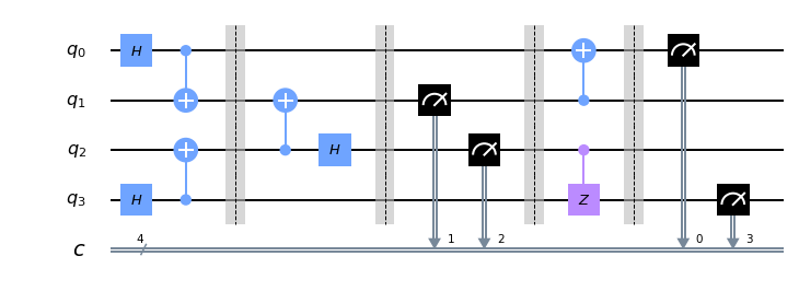
xxxxxxxxxx
 
 
 
 
 
 
 
backend = Aer.get_backend('qasm_simulator')
 
 
job_sim = execute(qc, backend, shots=4096*8)
 
sim_result = job_sim.result()
 

 
measurement_result = sim_result.get_counts(qc)
 

 
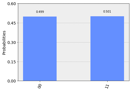
traced_result = {'00':0, '11':0}
 
for v, k in measurement_result.items():
 
    res = 0
 
    if v[0] == '0':
 
        res = traced_result['00'] + k
 
        traced_result.update({'00':res})
 
    else:
 
        res = traced_result['11'] + k
 
        traced_result.update({'11':res})
 

 
print(traced_result)
 
plot_histogram(traced_result)
 
 
 
 
 
 

xxxxxxxxxx
 
 
 
 
 
 
{'00': 16343, '11': 16425}
 
 
 
 
 
 

 

 

 

The really important thing to realize is that, after that Bell basis measurement, Alice and Carol could be in one of many possible entangled states. Their qubits might be entangled to agree along the $X$$X$ axis, or to disagree. They also might agree or disagree along the $Z$$Z$ axis. Concretely speaking, they could be in the state $|00⟩+|11⟩$$|00\rangle + |11\rangle$, or in the state $|01⟩+|10⟩$$|01\rangle + |10\rangle$, or in the state $|00⟩-|11⟩$$|00\rangle - |11\rangle$, or in the state $|01⟩-|10⟩$$|01\rangle - |10\rangle$.

But then there's still Bob's measurement results. They reveal which entangled case Alice and Carol ended up in. Bob knows their state's X-parity and its Z-parity. All Bob has to do is tell Alice and Carol "Hey, the Z-parity came out 'disagree' so one of you flip your qubit 180 degrees around the X axis to fix that". Do the same for the X-parity, and the problem is solved: Alice and Carorl will definitely end up in the state $|00⟩+|11⟩$$|00\rangle + |11\rangle$ after the corrections. Therefore, although Alice and Carol never interacted with each other, their particles are now entangled.