Introduction to Quantum Machine Learning
A short review of the theory and motivation behind interlinking of quantum computing and machine learning.
Introduction
Models, simulations, and experiments have been at the forefront of research in both technology and natural sciences because of the large amount of data they produce. Extraction and processing of this large amount of data have been possible due to our advances towards more complex and powerful computational capabilities. These include implementation of linear algebraic techniques such as regression, principal component analysis, support vector machines, development of statistical frameworks such as Markov chains, and the emergence of novel machine learning and deep learning methods such as artificial neural networks (perceptrons), convolutional neural network (CNN), and Boltzmann machines.
In the past decade, these techniques have been extensively used in large datasets in both industries and academic research. In fact, a large number of HPCs (with GPUs, TPUs, etc.) have used their billions of clock cycles to train deep learning networks on useful datasets to identify complex and subtle patterns in data. These have resulted in the development of computational programs useful in disease classification in clinical diagnosis, new materials and compounds discovery, path planning in autonomous robots, etc. However, training these networks to do something useful takes a lot of computational resources depending on the complexity of the task at hand. This is because classical/deep machine learning methods either require algebraic routines (SVM, PCA, etc), recognizing statistical patterns in data (deep neural networks) and often both. As we will be studying below, this observation leads to a hope that quantum computing could be a way forward in improvement, but before jumping there, let us first briefly revisit quantum computers.
A quantum computational device uses quantum mechanical resources such as superposition, entanglement, and tunneling to gain a possible computational advantage over classical processors, also known as quantum speedup. In the last couple of years, there has been successful development and demonstration of quantum processors by IBM, Rigetti, Google, etc. However, the computational capabilities of these current generation quantum processors also known as Noisy Intermediate-Scale Quantum (NISQ) devices, are considerably restricted due to their intermediate size (in terms of qubits count), limited connectivity, imperfect qubit-control, short coherence time and minimal error-correction. Nevertheless, they can still be used with a classical computer as an accelerator, to solve those parts of the problem which are intractable for classical computers. This will be discussed further in Section-2.
Therefore, even though fault-tolerant quantum computers are still years away, the field has already left the purely academic sphere and is on the agenda of industries like us. Now, coming back to using the current generation quantum computers in machine learning, it must be noted that their success depends on whether an efficient quantum algorithm (such as QBoost) can be found for this task. This idea is being explored under a collaborative framework of Quantum Machine Learning (QML), a term popularised by Lloyd, Mohseni and Rebentrost (2013), and Peter Wittek (2014). In general, there are multiple definitions of this term based on the approach followed to integrate both quantum computing and machine learning, depending upon data generation and data processing systems – Quantum (Q) and Classical (C). These approaches are represented neatly in Figure 1.
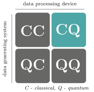
Figure 1. Four approaches that combine quantum computing and machine learning. The case CC refers to classical data being processed classically, and the case QC refers to using classical machine learning in quantum computing. Here, we focus on CQ and QQ approaches in which we use quantum computing devices to process both quantum and classical data. [2]
In this article, we will be mainly focusing on the CQ and QQ approach, where quantum computing is used on both classical and quantum (i.e. data generated from quantum experiments, simulations, sensors, etc.) data respectively. Moreover, depending upon how quantum computers are used to attain a quantum speedup in a classical/deep learning algorithm we have defined two waves in QML. Algorithms proposed in the first wave required fault-tolerance quantum devices and qRAM, whereas, the second wave algorithms can be run on NISQ devices and don’t require qRAM. The rest of the article is divided into 5 Sections – In Section I and Section II, we discuss the first and second wave of QML. In Section III, we discuss the promising application of QML in the industry, and finally, in Section IV we discuss our plans in the field.
The First Wave of Quantum Machine Learning
The first wave in QML started in 2010 when theoretical quantum algorithms like QSVM, QPCA, QBoost, Q-Means, etc. were proposed. These algorithms were aimed towards speeding ML, and hence required the existence of both fault-tolerant quantum devices and QRAM to attain a quantum advantage. We have listed down the motivation and promises of the algorithms put forward in the first wave in Table I and Table II respectively.
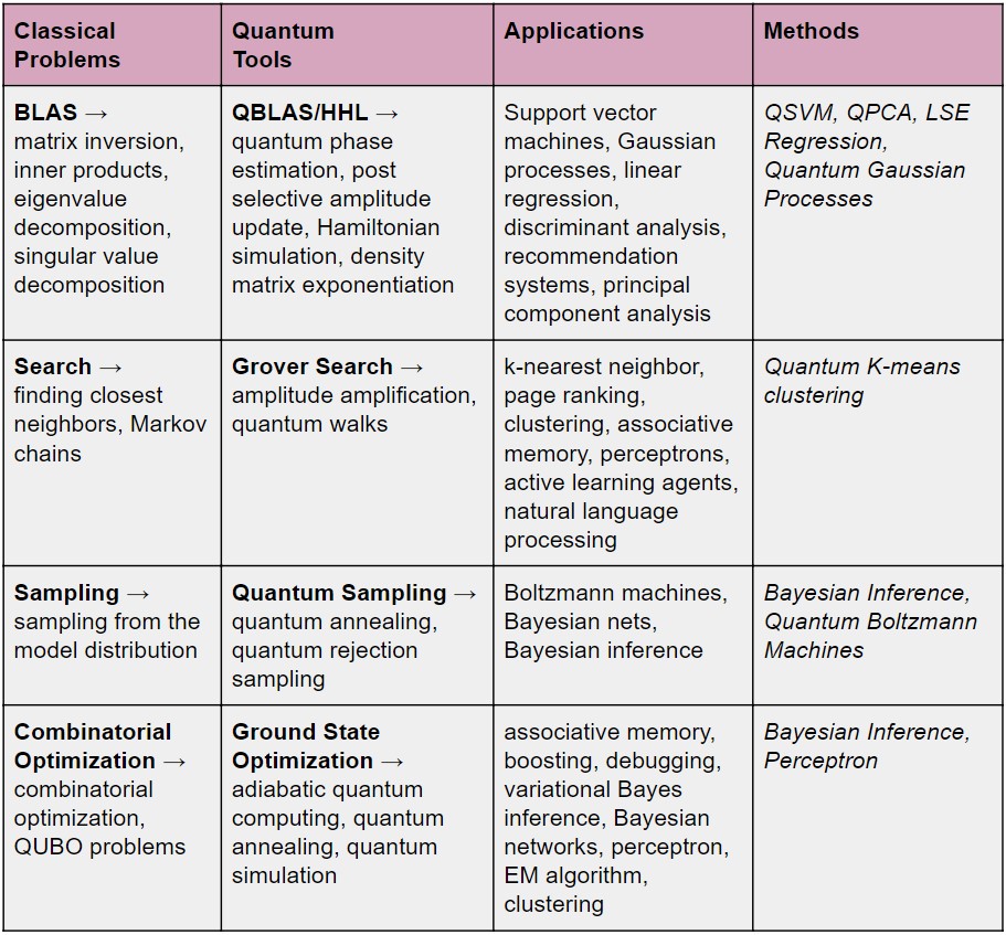
Table 1: Quantum alternatives to solve classical problems.
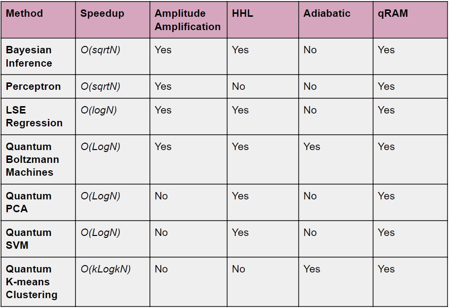
Table 2: Quantum speedup achieved in different methods [1]
Caveats in the Proposal
Proposals of these algorithms did heat the quantum research community. However, there were certain caveats in their success:
-
Fault-tolerance – Since most of these algorithms require methods like HHL, they were not feasible on near-term quantum processors.
-
QRAM – It might be possible that an advantageous QRAM might not be possible. Hence, for most of these algorithms, the advantage gained during computation on quantum devices could be nullified by the cost incurred during the data encoding/loading procedure.
-
Dequantization – Ewin Tang presented quantum-inspired classical algorithms for recommendation systems, low-rank HHL, PCA, etc. that essentially gave the same performance as the quantum algorithms.
The Second Wave of Quantum Machine Learning
The successful development and demonstration of quantum hardware in 2016 initiated the second wave quantum machine learning, which is currently in progress. Till now, the proposed candidates are hybrid quantum-classical heuristics. These involve using limited-depth parameterized quantum circuits on NISQ processors to prepare highly entangled quantum states, and then application of classical optimization routine for tuning parameters to converge to the target quantum state. Such a hybrid quantum-classical approach is represented in Figure 2.
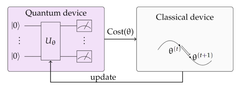
Figure 2. In the hybrid quantum-classical paradigm, the quantum computer prepares quantum states according to a set of parameters. Measurement outcomes from this state are used to calculate cost on the classical device. It then makes use of learning algorithms and adjusts the parameters in order to minimize the cost. The updated parameters are then fed back to the quantum hardware completing the feedback loop. [8]
The first important quantum method of learning used the quantum Ising model to train Boltzmann machines and Hopfield models. This integration of traditional machine learning with quantum computing lead to better convergence in such models. On the other hand, the current most popular methods of learning are hybrid algorithms. One basic example of these could be the variational algorithms, which are based on the variational principle of quantum mechanics. In this algorithm, the problem is encoded in a hermitian operator M such as Hamiltonian. Then a trial wavefunction is prepared using the state preparation circuit, which acts as our guess answer state. Next, we use a parameterized circuit known as an ansatz to evolve this trial wavefunction. A classical processor then performs measurements to evaluate the expectation value of M, and tune the ansatz parameters. These parameters are optimized such that they evolve our initially prepared state to the target wavefunction which minimized the expectation value of M. A variational paradigm of training ML is given in Figure 2, and a few examples of the ansatz used in the variational circuits are given in Figure 3

Figure 3. Ansatz in the variational paradigm can be segregated into two parts: A – state evolver and B – state entangler. The first part A consists of single unitary gates and evolves the state fed to it via state preparatory circuit. The second part B consists of both single and two-qubit gates. This introduces the entanglement between the qubits. In short, for any ansatz by parameterizing these two parts either individually or together let us tune its expressibility i.e. the states it could cover in Hilbert space and its entangling capability i.e. the measure of entanglement in the evolved state. Therefore, in order to choose good ansatz, its template is decided based on the problems in hand (problem-based ansatz) and hardware being used (hardware efficient ansatz). [4]
These hybrid approaches based on parameterized quantum circuits (PQCs) have been demonstrated to perform incredibly well on machine learning tasks such as classification, regression, and generative modeling. This success is easier to explain if we notice the similarities between PQCs and classical models, such as neural networks and kernel methods. The similarity with both of these methods could be by the representation given in Figure 4.
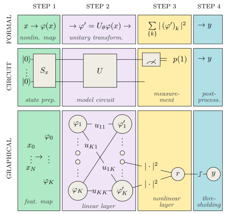
Figure 4. The quantum circuit utilized in variational paradigm can be realized in the three ways: a formal mathematical framework, a quantum circuit framework, and a graphical neural network framework. In the first step, we encode our data into the quantum state i.e. our feature vector, using a state preparation scheme. The quantum circuit then evolves this state using unitary operations. This could be thought of as the linear layers of a neural network. Measurements present in the next step effectively implements the weightless nonlinear layer. Finally, at the post processing step, we evaluate the thresholding function to produce a binary output. [4]
Moreover, in the recent research literature, there has been a lot of work regarding computing the partial derivative of quantum expectation values with respect to the gate parameters through procedures such as parameter shift rule. The development of these results has allowed some important advancement in the field of QML, such as gradient-based optimization strategies. This ability to compute quantum gradients means that quantum computations are now compatible with techniques such as backpropagation, which is an important procedure in deep learning. Moreover, this allows the development of automatically differentiable hybrid networks, which involves both quantum and classical nodes. Such a pipeline has been represented in figure 5 with calculations of gradients using parameter shift rule.
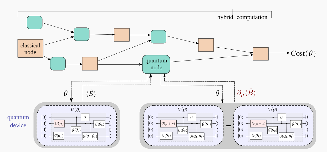
Figure 5. In the hybrid computation paradigm we can build networks that consist of both quantum (orange) and classic (blue) nodes. In such networks, an output from a classical node is fed to the quantum node on which it executes a variational quantum algorithm and finds the expectation value of the operator B depending on parameters θ. Here, we show the parameter shift rule, which allows us to compute the derivative of the quantum node by executing the circuit twice, but with a shift (𝜇±s) in the parameter with respect to which the derivative is calculated. [9]
Apart from such classically-parametrized quantum routines, there also has been considerable work done in developing quantumly-parametrized networks. To train these types of networks we make use of quantum mechanical phenomena such as quantum tunneling, phase kickbacks to get information regarding gradients. Thus, this allows for quantum-enhanced optimization techniques such as Quantum Dynamical Descent (QDD) and Momentum Measurement Gradient Descent (MoMGrad) to train parameters of these hybrid/quantum networks. Similarly, for meta-training, i.e., the quantum hyper-parameter training of such a hybrid/quantum network, variants of these algorithms such as Meta-QDD and Meta-MoMGrad have been proposed as quantum meta-learning methods. These methods rely on producing entanglement between the quantum hyper-parameters in superposition. Detailed discussion on these techniques is given in [10].
Applications
Till now, we have learned that being in the middle of the second wave of QML, our best bet is hybrid approaches. These involve training parameterized quantum circuit models for a variety of supervised and unsupervised machine learning tasks on both classical and quantum data. In general, a few examples of these tasks could be:
-
Recognizing patterns to classify classical data.
-
Learning the probability distribution of the training data and generate new data following similar probability distribution.
-
Finding short-depth hardware-efficient circuits for high-level algorithms.
-
Compression of the quantum states.
These tasks enable using quantum machine learning in a variety of fields ranging from chemical simulations, combinatorial optimizations, finance, quantum many-body simulations, the energy sector, healthcare sector, etc.
References
-
Jacob Biamonte, Peter Wittek, et al., Quantum Machine Learning, 1611.09347
-
Brassard, et al., Machine learning in a quantum world. In: Advances in Artificial Intelligence, Springer 2006
-
Farhi & Neven, Classification with Quantum Neural Networks on Near Term Processors, 1802.06002,
-
Schuld et al., Circuit-centric quantum classifiers, 1804.00633
-
Benedetti et al., Parameterized quantum circuits as machine learning models, 1906.07682
-
Schuld & Petruccione, Supervised Learning with Quantum Computers, Springer 2018
-
Guerreschi & Smelyanskiy, Practical optimization for hybrid quantum-classical algorithms, 1701.01450
-
Mitarai et al., Quantum Circuit Learning, 1803.00745
-
Schuld et al., Evaluating analytic gradients on quantum hardware, 1811.11184
-
Guillaume Verdon et al., A Universal Training Algorithm for Quantum Deep Learning, 1806.09729