Building Variational Quantum Eigensolver from scratch

Let us assume that we are given a $2^N\times 2^N$$2^N\times2^N$ dimension matrix (like the one given below).

Today, we will be finding eigenvalues of such matrices using VQE-like circuits for such matrices. While doing so, we will cover the following topics:

1. Hamiltonian in Pauli Basis
2. Calculations of Expectation Value
3. Designing Ansatze
4. Running Simulations
5. Running Noisy Simulations
6. Extension to Excited Energy States
7. Interpreting the Results

Necessary Imports

xxxxxxxxxx
import numpy as np
import scipy as sp
import itertools
import functools as ft
%matplotlib notebook
import matplotlib.pyplot as plt
from mpl_toolkits import mplot3d
import re 

xxxxxxxxxx
#!pip install qiskit
from qiskit import *
from qiskit.providers.aer.noise import NoiseModel
from qiskit.providers.aer.noise import QuantumError, ReadoutError
from qiskit.providers.aer.noise import phase_amplitude_damping_error
from qiskit.providers.aer.noise import depolarizing_error
from qiskit.providers.aer.noise import thermal_relaxation_error
from qiskit.ignis.mitigation.measurement import complete_meas_cal, CompleteMeasFitter

Hamiltonian in Pauli Basis

The normalized Pauli matrices $\{{\sigma }_0,{\sigma }_x,{\sigma }_y,{\sigma }_z\}/\sqrt{2}$$\{\sigma_0,\sigma_x,\sigma_y,\sigma_z\}/{\sqrt{2}}$ form an orthogonal basis of ${\mathcal{M}}_2$$\mathcal{M}_2$, this vector space can be endowed with a scalar product called the Hilbert-Schmidt inner product: $⟨A,B⟩=Tr(A^{†}B)$$⟨A,B⟩=Tr(A^{\dagger}B)$. Since the Pauli matrices anticommute, their product is traceless, and since they are Hermitian this implies that they are orthogonal with respect to that scalar product. Hence this property can be used for decomposing a Hamiltonian as:

$H=\sum _{i_1,\dots ,i_n=\{0,x,y,z\}}{h}_{i_1,\dots ,i_n}\cdot \frac{1}{2^n}{\sigma }_{i_1}\otimes \dots \otimes {\sigma }_{i_n}$$H = \sum_{i_{1},\ldots,i_{n} = \{0,x,y,z\}}h_{i_{1},\ldots,i_{n}}\cdot \frac{1}{2^{n}}\sigma_{i_1}\otimes\ldots\otimes\sigma_{i_n}$

$h_{i_1,\dots ,i_n}=\frac{1}{2^n}\text{Tr}(({\sigma }_{i_1}\otimes \dots \otimes {\sigma }_{i_n}{)}^{†}\cdot H)=\frac{1}{2^n}\text{Tr}(({\sigma }_{i_1}\otimes \dots \otimes {\sigma }_{i_n})\cdot H)$$h_{i_{1},\ldots,i_{n}} = \frac{1}{2^{n}}\text{Tr}\big((\sigma_{i_1}\otimes\ldots\otimes\sigma_{i_n})^\dagger \cdot H\big) = \frac{1}{2^{n}}\text{Tr}\big((\sigma_{i_1}\otimes\ldots\otimes\sigma_{i_n}) \cdot H\big)$

Decomposing Hamiltonian into Pauli Terms

xxxxxxxxxx
def decompose_ham_to_pauli(H):
    """Decomposes a Hermitian matrix into a linear combination of Pauli operators.

    Args:
        H (array[complex]): a Hermitian matrix of dimension 2**n x 2**n.

    Returns:
        tuple[list[float], list[string], list [ndarray]]: a list of coefficients, 
        a list of corresponding string representation of tensor products of Pauli 
        observables that decompose the Hamiltonian, and
        a list of their matrix representation as numpy arrays
    """

    n = int(np.log2(len(H)))
    N = 2 ** n

    # Sanity Checks
    if H.shape != (N, N):
        raise ValueError(
            "The Hamiltonian should have shape (2**n, 2**n), for any qubit number n>=1"
        )

    if not np.allclose(H, H.conj().T):
        raise ValueError("The Hamiltonian is not Hermitian")

    sI = np.eye(2, 2, dtype=complex)
    sX = np.array([[0, 1], [1, 0]], dtype=complex)
    sZ = np.array([[1, 0], [0,-1]], dtype=complex)
    sY = complex(0,-1)*np.matmul(sZ,sX)
    paulis = [sI, sX, sY, sZ]
    paulis_label = ['I', 'X', 'Y', 'Z']
    obs = []
    coeffs = []
    matrix = []
    
    for term in itertools.product(paulis, repeat=n):
        matrices = [pauli for pauli in term]
        coeff = np.trace(ft.reduce(np.kron, matrices) @ H) / N 
        coeff = np.real_if_close(coeff).item()
        
        # Hilbert-Schmidt-Product
        if not np.allclose(coeff, 0): 
            coeffs.append(coeff)
            obs.append(''.join([paulis_label[[i for i, x in enumerate(paulis) 
            if np.all(x == t)][0]]+str(idx) for idx, t in enumerate(reversed(term))]))
            matrix.append(ft.reduce(np.kron, matrices))

    return obs, coeffs , matrix

Composing Hamiltonian into Pauli Terms

xxxxxxxxxx
def compose_ham_from_pauli(terms, coeffs):
    """Composes a Hermitian matrix from a linear combination of Pauli operators.

    Args:
        tuple[list[float], list[string]]: a list of coefficients, 
        a list of corresponding string representation of tensor products of 
        Pauli observables that decompose the Hamiltonian.

    Returns:
        H (array[complex]): a Hermitian matrix of dimension 2**n x 2**n.
    """

    pauli_qbs = [re.findall(r'[A-Za-z]|-?\d+\.\d+|\d+', x) for x in terms]
    qubits = max([max(list(map(int, x[1:][::2]))) for x in pauli_qbs])

    N = int(2**np.ceil(np.log2(qubits+1)))

    sI = np.eye(2, 2, dtype=complex)
    sX = np.array([[0, 1], [1, 0]], dtype=complex)
    sZ = np.array([[1, 0], [0,-1]], dtype=complex)
    sY = complex(0,-1)*np.matmul(sZ,sX)
    paulis = [sI, sX, sY, sZ]
    paulis_label = ['I', 'X', 'Y', 'Z']
    paulis_term = {'I':sI, 'X':sX, 'Y':sY, 'Z':sZ}
    hamil = np.zeros((2**N, 2**N), dtype=complex) 

    for coeff, pauli_qb in zip(coeffs, pauli_qbs):
      term_str = ['I'] * N
      for term, index in zip(pauli_qb[0:][::2], pauli_qb[1:][::2]):
        term_str[int(index)] = term
      matrices = [paulis_term[pauli] for pauli in term_str]
      term_matrix = np.asarray(ft.reduce(np.kron, matrices[::-1]))
      hamil += coeff*term_matrix
    
    # Sanity Check
    if not np.allclose(hamil, hamil.conj().T):
        raise ValueError("The Hamiltonian formed is not Hermitian")

    return hamil

Test Hamiltonian

xxxxxxxxxx
H0 = np.array([
                [ 0.7056    ,  0.         , -0.       ,  0.        ],
                [ 0.        ,  -1.1246    , 0.182     ,  0.        ],
                [-0.        , 0.182       ,  0.4318   , -0.        ],
                [ 0.        ,  0.         , -0.       ,  0.888     ]
               ])
H0

xxxxxxxxxx
array([[ 0.7056,  0.    , -0.    ,  0.    ],
       [ 0.    , -1.1246,  0.182 ,  0.    ],
       [-0.    ,  0.182 ,  0.4318, -0.    ],
       [ 0.    ,  0.    , -0.    ,  0.888 ]])

xxxxxxxxxx
a, b , c = decompose_ham_to_pauli(H0)
a, b

xxxxxxxxxx
(['I0I1', 'Z0I1', 'X0X1', 'Y0Y1', 'I0Z1', 'Z0Z1'],
 [0.2252, 0.3435, 0.091, 0.091, -0.43470000000000003, 0.5716])

$H_0=0.2252\times I_0{I}_1+0.3435\times Z_0-0.4347\times Z_1+0.91\times X_0{X}_1+0.91\times Y_0{Y}_1+0.5716\times Z_0{Z}_1$$H_{0} = 0.2252\times I_{0}I_{1} + 0.3435\times Z_{0} - 0.4347\times Z_{1} + 0.91\times X_{0}X_{1} + 0.91\times Y_{0}Y_{1} + 0.5716 \times Z_{0}Z_{1}$

xxxxxxxxxx
compose_ham_from_pauli(a, b)

xxxxxxxxxx
array([[ 0.7056+0.j,  0.    +0.j,  0.    +0.j,  0.    +0.j],
       [ 0.    +0.j, -1.1246+0.j,  0.182 +0.j,  0.    +0.j],
       [ 0.    +0.j,  0.182 +0.j,  0.4318+0.j,  0.    +0.j],
       [ 0.    +0.j,  0.    +0.j,  0.    +0.j,  0.888 +0.j]])

xxxxxxxxxx
assert(np.isclose(compose_ham_from_pauli(a, b).real, H0).all())

Given Hamiltonian

xxxxxxxxxx
H1 = np.array([[1, 0, 0, 0], 
             [0, 0, -1, 0], 
             [0, -1, 0, 0], 
             [0, 0, 0, 1]])
H1

array([[ 1,  0,  0,  0],
       [ 0,  0, -1,  0],
       [ 0, -1,  0,  0],
       [ 0,  0,  0,  1]])

xxxxxxxxxx
a, b, c = decompose_ham_to_pauli(H1)
a, b

xxxxxxxxxx
(['I0I1', 'X0X1', 'Y0Y1', 'Z0Z1'], [0.5, -0.5, -0.5, 0.5])

$ H_{1} = 0.5\times (I_{0}I_{1} - X_{0}X_{1} - Y_{0}Y_{1} + Z_{0}Z_{1})$

xxxxxxxxxx
compose_ham_from_pauli(a, b)

xxxxxxxxxx
array([[ 1.+0.j,  0.+0.j,  0.+0.j,  0.+0.j],
       [ 0.+0.j,  0.+0.j, -1.+0.j,  0.+0.j],
       [ 0.+0.j, -1.+0.j,  0.+0.j,  0.+0.j],
       [ 0.+0.j,  0.+0.j,  0.+0.j,  1.+0.j]])

xxxxxxxxxx
assert(np.isclose(compose_ham_from_pauli(a, b).real, H1).all())

Calculating the Expectation values

For an $n$$n$-qubit quantum state, measuring one qubit corresponds to projecting the quantum state onto one of two half-spaces determined by the unique eigenvalues of our measurement operator.

By convention, performing a computational basis measurement is equivalent to measuring in measuring Pauli Z, which gives us two eigenvectors $|0⟩$$|0\rangle$ and $|1⟩$$|1\rangle$, with corresponding eigenvalues $\pm 1$$\pm 1$. Therefore, doing a computation measurement of a qubit and obtaining $0$$0$ means the state of our qubit is in the $+1$$+1$ eigenstate of the $Z$$Z$ operator. In general, we can then use the definition of the tensor product to perform multi-qubit measurements as will be explained below.

For some qubit $|\psi ⟩$$|\psi\rangle$ we have $|\psi ⟩=\alpha |0⟩+\beta |1⟩$$|\psi\rangle = \alpha |0\rangle + \beta|1\rangle$, we can calculate expectation value of a single-qubit operator $M=\sum _{m}m|m⟩⟨m|$$M = \sum_m m|m\rangle\langle m|$, as $⟨M⟩=⟨\psi |\sum _{m}m|m⟩⟨m|\psi ⟩=\sum _{m}m⟨\psi |m^{†}m|\psi ⟩=\sum _{m}mp(m)=(+1)p(0)+(-1)p(1)=p(0)-p(1)$$\langle M \rangle = \langle \psi | \sum_{m} m|m\rangle\langle m| \psi\rangle = \sum_m m \langle \psi |m^{\dagger} m| \psi\rangle = \sum_m m\space p(m) = (+1)p(0) + (-1)p(1) = p(0)-p(1)$. Similarly, for a two-qubit operator $M$$M$ we will get $⟨M⟩=p(00)+p(11)-p(01)-p(10)$$\langle M \rangle = p(00) + p(11) - p(01) - p(10)$.

Change of Basis

Therefore, to measure a qubit, we can use any $2\times 2$$2\times2$ operator that is a unitary transformation of $Z$$Z$. That is, we could also use a measurement operator $M=U^{†}ZU$$M=U^{\dagger}ZU$, where $U$$U$ is an unitary operator and $M$$M$ gives two unique outcomes of a measurement in its $\pm 1$$\pm 1$ eigenvectors. Thereofre, to measure in a basis other than the computational (or $Z$$Z$), we need to find the corresponding unitary equivalence. Similar to the one-qubit case, all two-qubit Pauli-measurements can be written as $(U_1^{†}\otimes U_2^{†})[Z\otimes Z](U_1\otimes U_2)$$(U_{1}^{\dagger}\otimes U_{2}^{\dagger}) [Z\otimes Z] (U_{1}\otimes U_{2})$ for $2\times 2$$2\times 2$ unitary matrices $U_1$$U_1$ and $U_2$$U_2$.

For $X$$X$, and $Y$$Y$ basis measurements, these unitary equivalence are given below:

$X=(H{)}^{†}ZH$$X = (H)^{\dagger} Z H$ $Y=(H{S}^{†}{)}^{†}Z(H{S}^{†})$$Y = (HS^{\dagger})^{\dagger} Z (HS^{\dagger})$

This feature can be exploited to create circuits for both $X$$X$ basis and $Y$$Y$ basis measurements from the standard $Z$$Z$ basis. It is done by applying the corresponding unitary operation to the prepared quantum state and then performing a measurement in $Z$$Z$ basis.

For example: In order to do a $Y$$Y$ basis measurement, first apply $H{S}^{†}$$HS^{\dagger}$ to the quantum state and then do a normal $Z$$Z$ basis measurement.

Similar to the one-qubit case, all multi-qubit Pauli-measurements can be written as a generalization of above.

For example: For two-qubit $X$$X$ basis measurement, $X\otimes X=(H\otimes H)[Z\otimes Z](H\otimes H)$$X\otimes X = (H\otimes H)[Z\otimes Z] (H\otimes H)$.

Constructing Measurement Circuits

xxxxxxxxxx
def measure_circuit(basis, num_qubits):
    """
    Generate measurement circuit according to the Pauli observable
    string provided. 

    Args:
    basis (str): String representation of tensor products of Pauli 
    observables
    num_qubits (int): Number of qubits in the circuit

    Returns:
    measure_qc (QuantumCircuit): Measurement Circuit for the 
    corresponding basis.
    
    """

    basis_qb = re.findall(r'[A-Za-z]|-?\d+\.\d+|\d+', basis)
    basis = basis_qb[0:][::2] 
    qubit = list(map(int, basis_qb[1:][::2]))

    measure_qc = QuantumCircuit(num_qubits, num_qubits)
    for base, qb in zip(basis, qubit):
      if base == 'I' or base == 'Z':
        pass
      elif base == 'X':
        measure_qc.h(qb)
      elif base == 'Y':
        measure_qc.sdg(qb)
        measure_qc.h(qb)
      else:
        raise ValueError("Wrong Basis provided")
    
    for qb in range(num_qubits):
        measure_qc.measure(qb, qb)

    return measure_qc

xxxxxxxxxx
def calculate_expecation_val(circuit, basis, shots=2048, backend='qasm_simulator'):
    """
    Calculate expectation value for the measurement of a circuit in a 
    given basis.

    Args:
    circuit (QuantumCircuit): Circuit using which expectation value 
    will be calculated for a given basis.
    basis (str): String representation of tensor products of Pauli 
    observables.
    shots (int): Number of times measurements needed to be done for calculating
    probability.
    backend (str): Backend for running the circuit.

    Returns:
    exp (float): Expectation value for the measurement of a circuit 
    in a given basis.

    """
    exp_circuit = circuit + measure_circuit(basis, circuit.num_qubits)

    result = execute(exp_circuit, backend=Aer.get_backend(backend),
                    shots=shots).result()
    
    exp = 0.0
    for key, counts in result.get_counts().items():
        exp += (-1)**(int(key[0])+int(key[1])) * counts

    return exp/shots

Examples

Measurements in XX, YY, ZZ basis

xxxxxxxxxx
measure_circuit('X0X1', 2).draw()

     ┌───┐┌─┐   
q_0: ┤ H ├┤M├───
     ├───┤└╥┘┌─┐
q_1: ┤ H ├─╫─┤M├
     └───┘ ║ └╥┘
c: 2/══════╩══╩═
           0  1 

xxxxxxxxxx
measure_circuit('Y0Y1', 2).draw()

     ┌─────┐┌───┐┌─┐   
q_0: ┤ SDG ├┤ H ├┤M├───
     ├─────┤├───┤└╥┘┌─┐
q_1: ┤ SDG ├┤ H ├─╫─┤M├
     └─────┘└───┘ ║ └╥┘
c: 2/═════════════╩══╩═
                  0  1 

xxxxxxxxxx
measure_circuit('Z0Z1', 2).draw()

     ┌─┐   
q_0: ┤M├───
     └╥┘┌─┐
q_1: ─╫─┤M├
      ║ └╥┘
c: 2/═╩══╩═
      0  1 

Measurements in XY, YZ, ZX basis (To show flexibility of the function)

xxxxxxxxxx
measure_circuit('X0Y1', 2).draw()

      ┌───┐      ┌─┐   
q_0: ─┤ H ├──────┤M├───
     ┌┴───┴┐┌───┐└╥┘┌─┐
q_1: ┤ SDG ├┤ H ├─╫─┤M├
     └─────┘└───┘ ║ └╥┘
c: 2/═════════════╩══╩═
                  0  1 

xxxxxxxxxx
measure_circuit('Y0Z1', 2).draw()

     ┌─────┐┌───┐┌─┐
q_0: ┤ SDG ├┤ H ├┤M├
     └─┬─┬─┘└───┘└╥┘
q_1: ──┤M├────────╫─
       └╥┘        ║ 
c: 2/═══╩═════════╩═
        1         0 

xxxxxxxxxx
measure_circuit('Z0X1', 2).draw()

          ┌─┐   
q_0: ─────┤M├───
     ┌───┐└╥┘┌─┐
q_1: ┤ H ├─╫─┤M├
     └───┘ ║ └╥┘
c: 2/══════╩══╩═
           0  1 

Determining the Ansatz

Designing Ansatze

Ansatze are simply a parameterized quantum circuits (PQC), which play an essential role in the performance of many variational hybrid quantum-classical (HQC) algorithms. Major challenge while designing an asatz is to choose an effective template circuit that well represents the solution space while maintaining a low circuit depth and number of parameters. Here, we make a choice of two ansatze, one randomly and another inspired from the given hint.

Ansatz 1 (Random Choice)

xxxxxxxxxx
def ansatz1(params, num_qubits): 
    """
    Generate an templated ansatz with given parameters

    Args:
    params (array[float]): Parameters to initialize the parameterized unitary.
    num_qubits (int): Number of qubits in the circuit.
    
    Returns:
    ansatz (QuantumCircuit): Generated ansatz circuit

    """

    ansatz = QuantumCircuit(num_qubits, num_qubits)
    params = params.reshape(2,2)
    
    for idx in range(num_qubits):
      ansatz.rx(params[0][idx], idx)
    
    ansatz.cnot(0, 1)

    for idx in range(num_qubits):
      ansatz.rz(params[1][idx], idx)

    return ansatz

ansatz1(np.random.uniform(-np.pi, np.pi, (2,2)), 2).draw()

     ┌─────────────┐     ┌──────────────┐
q_0: ┤ RX(0.74906) ├──■──┤ RZ(-0.10279) ├
     ├─────────────┤┌─┴─┐├─────────────┬┘
q_1: ┤ RX(0.40493) ├┤ X ├┤ RZ(-2.3803) ├─
     └─────────────┘└───┘└─────────────┘ 
c: 2/════════════════════════════════════
                                         

Ansatz 2 (From Hint)

xxxxxxxxxx
def ansatz2(params, num_qubits): 
    """
    Generate an templated ansatz with given parameters

    Args:
    params (array[float]): Parameters to initialize the parameterized unitary.
    num_qubits (int): Number of qubits in the circuit.
    
    Returns:
    ansatz (QuantumCircuit): Generated ansatz circuit

    """
    params = np.array(params).reshape(1)
    ansatz = QuantumCircuit(num_qubits, num_qubits)
    ansatz.h(0)
    ansatz.cx(0, 1)
    ansatz.rx(params[0], 0)

    return ansatz

ansatz2([np.pi], 2).draw()

     ┌───┐     ┌────────┐
q_0: ┤ H ├──■──┤ RX(pi) ├
     └───┘┌─┴─┐└────────┘
q_1: ─────┤ X ├──────────
          └───┘          
c: 2/════════════════════
                         

Running Simulations

Variational Quantum Eigensolver (VQE) is based on Rayleigh-Ritz variational principle. To perform VQE, the first step is to enocde the problem into a Hermitian matrix $M$$M$, whose expectation value w.r.t a trial wave function $|\psi (\theta )⟩$$|\psi(\theta)\rangle$ which is yielded by an ansatz $U(\theta )$$U(\theta)$, i.e., nothing but a unitary paramterized by $\{\overrightarrow{\theta }\}$$\{\vec{\theta}\}$.

Here, we optimize these parameters $\{\overrightarrow{\theta }\}$$\{\vec{\theta}\}$ using scipy.optimize library based on a cost function $C(\theta )$$C(\theta)$, which is nothing but the calculated expectation value of Hamiltonian, $H_1$$H_1$ for $|\psi (\theta )⟩$$|\psi(\theta)\rangle$: $C(\theta )=⟨\psi (\theta )|H_1|\psi (\theta )⟩$$C(\theta) = \langle \psi (\theta) | H_{1} | \psi (\theta) \rangle$

xxxxxxxxxx
def vqe(params, meas_basis, coeffs, circuit, num_qubits, shots=2048):
    """
        Return the calculated energy scalar for a given asnatz and 
        decomposed Hamiltoian. 

        Args:
        params (matrix(np.array)): Parameters for initializing the ansatz.
        meas_basis (list[str]): String representation of measurement basis, i.e.
        the decomposed pauli term with their corresponding qubits.
        coeffs (vector(np.array)): Coefficients for the decomposed Pauli Term
        circuit (QuantumCircuit): Template for Ansatz circuit 
        num_qubits (int): Number of qubits in the given asatze.
        shots (int): Number of shots to get the probability distribution.

        Return:
        energy (float): Expectation value of the Hamiltonian whose 
        decomposition was provided.
    """
    
    N = num_qubits
    circuit = circuit(params, num_qubits)
    energy = 0

    for basis, coeff in zip(meas_basis, coeffs):
      if basis.count('I') != N:
        energy += coeff*calculate_expecation_val(circuit, basis, shots)

    energy += 0.5

    return energy

Ansatz 1 (Random Choice)

xxxxxxxxxx
a, b, c = decompose_ham_to_pauli(H1)

params = np.random.uniform(-np.pi, np.pi, (2,2))
func = ft.partial(vqe, meas_basis=a, coeffs=b, circuit=ansatz1, 
                  num_qubits=2, shots=2048)

xxxxxxxxxx
res = sp.optimize.minimize(func, params, method='Powell')
res

xxxxxxxxxx
   direc: array([[1., 0., 0., 0.],
       [0., 1., 0., 0.],
       [0., 0., 1., 0.],
       [0., 0., 0., 1.]])
     fun: array(-1.)
 message: 'Optimization terminated successfully.'
    nfev: 190
     nit: 3
  status: 0
 success: True
       x: array([ 4.7130171 , -3.15044759, -1.59558296, -0.02529809])

xxxxxxxxxx
assert(float(res.fun) == min(np.linalg.eig(H1)[0])) #Sanity Check

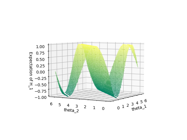
Visualizing the Result

After looking at multiple results' res.x, we realize that first and second parameters always have the values $\pm n\pi /2$$\pm n \pi/2$ and $\pm \pi$$\pm\pi$ respectively. So, while keeping them fixed, we do a parameters search-scan in the range ${\theta }_{3,4}\in [0,2\pi ]$$\theta_{3,4} \in [0,2\pi]$ and visualize how they affect our expectation value.

xxxxxxxxxx
def energy_expectation(x, y):
  """ Returns meshgrid values for plotting """
  energy = np.zeros(x.shape)
  for idx, thetas in enumerate(x):
    for ind, theta1 in enumerate(thetas):
      params = np.array([np.pi/2, np.pi, theta1, y[idx][ind]])
      energy[idx][ind] = func(params)
  return energy

theta1 = np.linspace(0.0, 2*np.pi, 200)
theta2 = np.linspace(0.0, 2*np.pi, 200)

X, Y = np.meshgrid(theta1, theta2)
Z = energy_expectation(X, Y)

fig = plt.figure()
ax = plt.axes(projection='3d')
ax.contour3D(X, Y, Z, 50, cmap='summer')
ax.set_xlabel('theta_1')
ax.set_ylabel('theta_2')
ax.set_zlabel('Expectation of H_1');
plt.show()

Ansatz 2 (From Hint)

xxxxxxxxxx
a, b, c = decompose_ham_to_pauli(H1)
params = np.random.uniform(-np.pi, np.pi, 1)
func = ft.partial(vqe, meas_basis=a, coeffs=b, circuit=ansatz2, 
                  num_qubits=2, shots=2048)

xxxxxxxxxx
res = sp.optimize.minimize(func, params, method='Powell')
res

xxxxxxxxxx
   direc: array([[1.]])
     fun: array(-1.)
 message: 'Optimization terminated successfully.'
    nfev: 26
     nit: 2
  status: 0
 success: True
       x: array([3.13590442])

xxxxxxxxxx
assert(float(res.fun) == min(np.linalg.eig(H1)[0])) #Sanity Check

Visualizing the Result

We scan over the paramter $\theta \in [0,2\pi ]$$\theta \in [0,2\pi]$, to visualize the change in expectation value for the ansatz2, which is inspired from the hint given.

xxxxxxxxxx
thetas = np.linspace(0.0, 2*np.pi, 500)
energy = np.zeros(len(thetas))

for idx, theta in enumerate(thetas):
    energy[idx] = func([theta])    

fig = plt.figure()
plt.plot(thetas, energy)
plt.title('Expectation value w.r.t angle theta')
plt.ylabel('Expectation value of $H_1$')
plt.xlabel('Theta (radians)')
indices = [idx for idx, x in enumerate(energy) if x <= -1.0]
xmin = thetas[indices[len(indices)//2]]
ymin = energy.min()
text= "Theta={:.3f}, \n Energy={:.3f}".format(xmin, ymin)
plt.plot(xmin,ymin,'x')
plt.annotate(text, xy=(xmin+0.75, ymin))
fig.show()

Number of Measurements (or Shots)

In order to obtain results from a quantum computer, one needs to perform sampling. This allows us to obtain the probability distribution, and hence know the most probable results from the measurement. Here, we see the change of expectation value of $H_1$$H_1$ with the number of shots, i.e., number of measurements for ansatz 2.

xxxxxxxxxx
thetas = np.linspace(0.0, 2*np.pi, 500)
shots = [128, 256, 512, 1024, 2048]
shot_energy = np.zeros((len(shots), len(thetas)))

for ind, shot in enumerate(shots):
    for idx, theta in enumerate(thetas):
        func = ft.partial(vqe, meas_basis=a, coeffs=b, circuit=ansatz2, 
                      num_qubits=2, shots=shot)
        shot_energy[ind][idx] = func([theta])    

xxxxxxxxxx
plt.figure()
for ind, shot in enumerate(shots):
    plt.plot(thetas, shot_energy[ind], label='Shots=' + str(shot))
    
plt.title('Expectation value w.r.t angle theta and shots')
plt.ylabel('Expectation value of $H_1$')
plt.xlabel('Theta (radians)')
plt.legend()
plt.show()

Performance of Classical Optimizers

Successful application of hybrid-quantum classical algorithms, with the classical step involving an optimizer, on current hardware, requires the classical optimizer to be noise-aware. In order to study this, we study the change of expectation value of $H_1$$H_1$ with different classical optimizers for ansatz 2, first in absence of noise, then later in the presence of noise.

xxxxxxxxxx
a, b, c = decompose_ham_to_pauli(H1)
params = np.random.uniform(-np.pi, np.pi, 1)
func = ft.partial(vqe, meas_basis=a, coeffs=b, circuit=ansatz2, 
                  num_qubits=2, shots=2048)

xxxxxxxxxx
optimizers = ['Nelder-Mead', 'L-BFGS-B', 'TNC', 'Powell', 'COBYLA', 'SLSQP']
opt_val = []
opt_param = []
opt_feval = []
opt_iter = []
init_params = params

for opt in optimizers:

    params = init_params
    res = sp.optimize.minimize(func, params, method=opt)

    opt_val.append(float(res.fun))
    opt_param.append(float(res.x))
    opt_feval.append(int(res.nfev))
    try:
        opt_iter.append(int(res.nit))
    except:
        opt_iter.append(1)

xxxxxxxxxx
fig = plt.figure()
plt.bar(optimizers, opt_val, color=['black', 'red', 'green', 'blue', 'yellow', 'orange'])
plt.title('Minimum expectation value w.r.t different optimizers')
plt.ylabel('Expectation value of $H_1$')
plt.xlabel('Optimizer')
plt.xticks(rotation=5)
fig.show()

xxxxxxxxxx
fig = plt.figure()
plt.bar(optimizers[:-1], opt_param[:-1], color=['black', 'red', 'green', 'blue', 'yellow'])
plt.title('Optimal parameter w.r.t different optimizers')
plt.ylabel('Value of theta')
plt.xlabel('Optimizer')
plt.xticks(rotation=5)
fig.show()

xxxxxxxxxx
fig = plt.figure()
plt.bar(optimizers[:-1], opt_feval[:-1], color=['black', 'red', 'green', 'blue', 'yellow'])
plt.title('Function evaluations w.r.t different optimizers')
plt.ylabel('Number of function evaluations$')
plt.xlabel('Optimizer')
plt.xticks(rotation=5)
fig.show()

xxxxxxxxxx
fig = plt.figure()
plt.bar(optimizers[:-1], opt_iter[:-1], color=['black', 'red', 'green', 'blue', 'yellow'])
plt.title('Number of iterations w.r.t different optimizers')
plt.ylabel('Number of iterations')
plt.xlabel('Optimizer')
plt.xticks(rotation=5)
fig.show()

Noisy Simulation

Computational power of NISQ processors suffers a lot from the limited capabilities of their physical qubits. This is essentially due to present of decoherence, limited connectivity, and absence of error-correction. Hence, it is essential to see how our ansatz would perform on a real device. Here, we replicate the noise model from a real device, and then test the perfrormance of our VQE module.

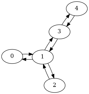
xxxxxxxxxx
# Noise Model Preparation
provider = IBMQ.load_account()
noisy_backend = provider.get_backend('ibmq_vigo')
coupling_map = noisy_backend.configuration().coupling_map
noise_model = providers.aer.noise.NoiseModel.from_backend(noisy_backend)
basis_gates = noise_model.basis_gates

Qubit coupling map of this real device is the following:

xxxxxxxxxx
qiskit.transpiler.CouplingMap(noisy_backend.configuration().coupling_map).draw()

xxxxxxxxxx
noise_model

xxxxxxxxxx
NoiseModel:
  Basis gates: ['cx', 'id', 'u2', 'u3']
  Instructions with noise: ['id', 'measure', 'cx', 'u2', 'u3']
  Qubits with noise: [0, 1, 2, 3, 4]
  Specific qubit errors: [('id', [0]), ('id', [1]), ('id', [2]), ('id', [3]), ('id', [4]), ('u2', [0]), ('u2', [1]), ('u2', [2]), ('u2', [3]), ('u2', [4]), ('u3', [0]), ('u3', [1]), ('u3', [2]), ('u3', [3]), ('u3', [4]), ('cx', [0, 1]), ('cx', [1, 0]), ('cx', [1, 2]), ('cx', [1, 3]), ('cx', [2, 1]), ('cx', [3, 1]), ('cx', [3, 4]), ('cx', [4, 3]), ('measure', [0]), ('measure', [1]), ('measure', [2]), ('measure', [3]), ('measure', [4])]

xxxxxxxxxx

def calculate_noisy_expecation_val(circuit, basis, mitigated=False, shots=2048, backend='qasm_simulator'):
    """
    Calculate expectation value for the measurement of a circuit in a 
    given basis in presence of noise.

    Args:
    circuit (QuantumCircuit): Circuit using which expectation value 
    will be calculated for a given basis.
    basis (str): String representation of tensor products of Pauli 
    observables.
    mitigated (bool): Whether mitigation has to be performed or not.
    shots (int): Number of times measurements needed to be done for calculating
    probability.
    backend (str): Backend for running the circuit.

    Returns:
    exp (float): Expectation value for the measurement of a circuit 
    in a given basis.

    """
    exp_circuit = circuit + measure_circuit(basis, circuit.num_qubits)
    
    result = execute(exp_circuit, backend=Aer.get_backend(backend),
                     shots=shots, coupling_map=coupling_map,
                     basis_gates=basis_gates,
                     noise_model=noise_model).result()

    if mitigated:
        meas_calibs, state_labels = complete_meas_cal(qr=exp_circuit.qregs[0], cr=exp_circuit.cregs[0])
        cal_results = qiskit.execute(meas_calibs, backend=Aer.get_backend(backend),
                                     coupling_map=coupling_map, basis_gates=basis_gates,
                                     shots=shots, noise_model=noise_model).result()
        meas_fitter = CompleteMeasFitter(cal_results, state_labels)
        meas_filter = meas_fitter.filter
        result = meas_filter.apply(result)
        
    exp = 0.0
    for key, counts in result.get_counts().items():
        exp += (-1)**(int(key[0])+int(key[1])) * counts

    return exp/shots


def noisy_vqe(params, meas_basis, coeffs, circuit, num_qubits, mitigated=False, shots=2048):
    """
        Return the calculated energy scalar for a given asnatz and 
        decomposed Hamiltoian in presence of noise. 

        Args:
        params (matrix(np.array)): Parameters for initializing the ansatz.
        meas_basis (list[str]): String representation of measurement basis, i.e.
        the decomposed pauli term with their corresponding qubits.
        coeffs (vector(np.array)): Coefficients for the decomposed Pauli Term
        circuit (QuantumCircuit): Template for Ansatz circuit 
        num_qubits (int): Number of qubits in the given asatze.
        mitigated (bool): Whether mitigation has to be performed or not.
        shots (int): Number of shots to get the probability distribution.

        Return:
        energy (float): Expectation value of the Hamiltonian whose 
        decomposition was provided.
    """
    
    N = num_qubits
    circuit = circuit(params, num_qubits)
    energy = 0

    for basis, coeff in zip(meas_basis, coeffs):
      if basis.count('I') != N:
        energy += coeff*calculate_noisy_expecation_val(circuit, basis, mitigated, shots)

    energy += 0.5

    return energy

Ansatz 1 (Random Choice)

xxxxxxxxxx
a, b, c = decompose_ham_to_pauli(H1)

params = np.random.uniform(-np.pi, np.pi, (2,2))
func = ft.partial(noisy_vqe, meas_basis=a, coeffs=b, circuit=ansatz1, 
                  num_qubits=2, mitigated=False, shots=8192)

xxxxxxxxxx
res = sp.optimize.minimize(func, params, method='Powell')
res

xxxxxxxxxx
   direc: array([[1., 0., 0., 0.],
       [0., 1., 0., 0.],
       [0., 0., 1., 0.],
       [0., 0., 0., 1.]])
     fun: array(-0.87451172)
 message: 'Optimization terminated successfully.'
    nfev: 266
     nit: 3
  status: 0
 success: True
       x: array([1.64212384, 3.14620703, 2.15383843, 0.53103981])

xxxxxxxxxx
a, b, c = decompose_ham_to_pauli(H1)

params = np.random.uniform(-np.pi, np.pi, (2,2))
func = ft.partial(noisy_vqe, meas_basis=a, coeffs=b, circuit=ansatz1, 
                  num_qubits=2, mitigated=True, shots=8192)

xxxxxxxxxx
res = sp.optimize.minimize(func, params, method='Powell')
res

xxxxxxxxxx
   direc: array([[1., 0., 0., 0.],
       [0., 1., 0., 0.],
       [0., 0., 1., 0.],
       [0., 0., 0., 1.]])
     fun: -0.9619728377818637
 message: 'Optimization terminated successfully.'
    nfev: 257
     nit: 3
  status: 0
 success: True
       x: array([ 1.58409174, -3.11397559, -0.50929574, -1.96419365])

Ansatz 2 (From Hint)

xxxxxxxxxx
a, b, c = decompose_ham_to_pauli(H1)
params = np.random.uniform(-np.pi, np.pi, 1)
func = ft.partial(noisy_vqe, meas_basis=a, coeffs=b, circuit=ansatz2, 
                  num_qubits=2, mitigated=False, shots=8192)

xxxxxxxxxx
res = sp.optimize.minimize(func, params, method='Powell')
res

xxxxxxxxxx
   direc: array([[-0.1127984]])
     fun: array(-0.88122559)
 message: 'Optimization terminated successfully.'
    nfev: 88
     nit: 5
  status: 0
 success: True
       x: array([3.17376448])

xxxxxxxxxx
a, b, c = decompose_ham_to_pauli(H1)
params = np.random.uniform(-np.pi, np.pi, 1)
func = ft.partial(noisy_vqe, meas_basis=a, coeffs=b, circuit=ansatz2, 
                  num_qubits=2, mitigated=True, shots=8192)

xxxxxxxxxx
res = sp.optimize.minimize(func, params, method='Powell')
res

xxxxxxxxxx
   direc: array([[3.01441921e-09]])
     fun: -0.9702586386528804
 message: 'Optimization terminated successfully.'
    nfev: 120
     nit: 5
  status: 0
 success: True
       x: array([-3.12601157])

Visualizing the Result (Noisy v/s Mitigated v/s Ideal)

xxxxxxxxxx
thetas = np.linspace(0.0, 2*np.pi, 500)
energy1 = np.zeros(len(thetas))
energy2 = np.zeros(len(thetas))
func1 = ft.partial(noisy_vqe, meas_basis=a, coeffs=b, circuit=ansatz2, 
                  num_qubits=2, mitigated=False, shots=8192)
func2 = ft.partial(noisy_vqe, meas_basis=a, coeffs=b, circuit=ansatz2, 
                  num_qubits=2, mitigated=True, shots=8192)

for idx, theta in enumerate(thetas):
    energy1[idx] = func1([theta])    
    energy2[idx] = func2([theta])    

xxxxxxxxxx
plt.plot(thetas, energy, label='simulation')
plt.plot(thetas, energy1, label='noisy')
plt.plot(thetas, energy2, label='mitigated')
plt.title('Expectation value w.r.t angle theta')
plt.ylabel('Expectation value of $H_1$')
plt.xlabel('Theta (radians)')
plt.legend()
plt.show()

xxxxxxxxxx
<IPython.core.display.Javascript object>

Number of Measurements (or Shots)

Let's see the change of expectation value of $H_1$$H_1$ with the number of shots for ansatz 2.

xxxxxxxxxx
thetas = np.linspace(0.0, 2*np.pi, 500)
shots = [128, 256, 512, 1024, 2048]
noisy_shot_energy = np.zeros((len(shots), len(thetas)))

for ind, shot in enumerate(shots):
    for idx, theta in enumerate(thetas):
        func = ft.partial(noisy_vqe, meas_basis=a, coeffs=b, circuit=ansatz2, 
                      num_qubits=2, shots=shot)
        noisy_shot_energy[ind][idx] = func([theta])    

xxxxxxxxxx
plt.figure()
for ind, shot in enumerate(shots):
    plt.plot(thetas, noisy_shot_energy[ind], label='Shots=' + str(shot))
    
plt.title('Expectation value w.r.t angle theta and shots')
plt.ylabel('Expectation value of $H_1$')
plt.xlabel('Theta (radians)')
plt.legend()
plt.show()

Peformance of Classical Optimizers

Let's see the change of expectation value of $H_1$$H_1$ with different classical optimizers for ansatz 2.

xxxxxxxxxx
a, b, c = decompose_ham_to_pauli(H1)
params = np.random.uniform(-np.pi, np.pi, 1)
func = ft.partial(noisy_vqe, meas_basis=a, coeffs=b, circuit=ansatz2, 
                  num_qubits=2, mitigated=True, shots=8192)

xxxxxxxxxx
optimizers = ['Nelder-Mead', 'L-BFGS-B', 'TNC', 'Powell', 'COBYLA', 'SLSQP']
opt_val = []
opt_param = []
opt_feval = []
opt_iter = []

init_params = params

for opt in optimizers:

    params = init_params
    res = sp.optimize.minimize(func, params, method=opt)

    opt_val.append(float(res.fun))
    opt_param.append(float(res.x))
    opt_feval.append(int(res.nfev))
    try:
        opt_iter.append(int(res.nit))
    except:
        opt_iter.append(1)

xxxxxxxxxx
fig = plt.figure()
plt.bar(optimizers, opt_val, color=['black', 'red', 'green', 'blue', 'yellow', 'orange'])
plt.title('Minimum expectation value w.r.t different optimizers')
plt.ylabel('Expectation value of $H_1$')
plt.xlabel('Optimizer')
plt.xticks(rotation=5)
fig.show()

xxxxxxxxxx
fig = plt.figure()
plt.bar(optimizers[:-1], opt_param[:-1], color=['black', 'red', 'green', 'blue', 'yellow'])
plt.title('Optimal parameter w.r.t different optimizers')
plt.ylabel('Value of theta')
plt.xlabel('Optimizer')
plt.xticks(rotation=5)
fig.show()

xxxxxxxxxx
fig = plt.figure()
plt.bar(optimizers[:-1], opt_feval[:-1], color=['black', 'red', 'green', 'blue', 'yellow'])
plt.title('Function evaluations w.r.t different optimizers')
plt.ylabel('Number of function evaluations')
plt.xlabel('Optimizer')
plt.xticks(rotation=5)
fig.show()

xxxxxxxxxx
fig = plt.figure()
plt.bar(optimizers[:-1], opt_iter[:-1], color=['black', 'red', 'green', 'blue', 'yellow'])
plt.title('Number of iterations w.r.t different optimizers')
plt.ylabel('Number of iterations')
plt.xlabel('Optimizer')
plt.xticks(rotation=5)
fig.show()

Comparing the performance of VQE in presence of errors due to Readout, Thermal Relaxation, Amplitude-Phase damping and Depolarization

Readout

Describes classical readout errors

xxxxxxxxxx
# Measurement miss-assignement probabilities
p0given1 = 0.1
p1given0 = 0.05
noise_readout = ReadoutError([[1 - p1given0, p1given0], [p0given1, 1 - p0given1]])
noise_readout

xxxxxxxxxx
ReadoutError([[0.95 0.05]
 [0.1  0.9 ]])

Thermal Relaxation

Single qubit thermal relaxation error is characterized by relaxation time constants $T_1$$T_1$, $T_2$$T_2$, and the gate time $t$$t$.

xxxxxxxxxx
num_qubits = 2

T1s = np.random.normal(50e3, 10e3, num_qubits) # Sampled from normal distribution
T2s = np.random.normal(80e3, 20e3, num_qubits)  # Sampled from normal distribution
T2s = np.array([min(T2s[j], 2 * T1s[j]) for j in range(num_qubits)]) # Ensuring T2s < 2*T1s

# Instruction times (in nanoseconds)
time_u1 = 0   # virtual gate
time_u2 = 50  # (single X90 pulse)
time_u3 = 100 # (two X90 pulses)
time_cx = 300
time_measure = 1000 # 1 microsecond

# Add depolarizing error to all single qubit u1, u2, u3, cx, measure gates
errors_thermal_u1  = [thermal_relaxation_error(t1, t2, time_u1)
              for t1, t2 in zip(T1s, T2s)]
errors_thermal_u2  = [thermal_relaxation_error(t1, t2, time_u2)
              for t1, t2 in zip(T1s, T2s)]
errors_thermal_u3  = [thermal_relaxation_error(t1, t2, time_u3)
              for t1, t2 in zip(T1s, T2s)]
errors_thermal_cx = [[thermal_relaxation_error(t1a, t2a, time_cx).expand(
             thermal_relaxation_error(t1b, t2b, time_cx))
              for t1a, t2a in zip(T1s, T2s)]
               for t1b, t2b in zip(T1s, T2s)]
errors_thermal_measure = [thermal_relaxation_error(t1, t2, time_measure)
                  for t1, t2 in zip(T1s, T2s)]

# Add errors to noise model
noise_thermal = NoiseModel()
for j in range(num_qubits):
    noise_thermal.add_quantum_error(errors_thermal_u1[j], "u1", [j])
    noise_thermal.add_quantum_error(errors_thermal_u2[j], "u2", [j])
    noise_thermal.add_quantum_error(errors_thermal_u3[j], "u3", [j])
    for k in range(num_qubits):
        noise_thermal.add_quantum_error(errors_thermal_cx[j][k], "cx", [j, k])
    noise_thermal.add_quantum_error(errors_thermal_measure[j], "measure", [j])

noise_thermal

xxxxxxxxxx
NoiseModel:
  Basis gates: ['cx', 'id', 'u2', 'u3']
  Instructions with noise: ['u2', 'u3', 'cx', 'measure']
  Qubits with noise: [0, 1]
  Specific qubit errors: [('u2', [0]), ('u2', [1]), ('u3', [0]), ('u3', [1]), ('cx', [0, 0]), ('cx', [0, 1]), ('cx', [1, 0]), ('cx', [1, 1]), ('measure', [0]), ('measure', [1])]

Amplitude-Phase Damping

Single-qubit generalized combined phase and amplitude damping error is given by an amplitude damping parameter $\lambda$$\lambda$, and a phase damping parameter $\gamma$$\gamma$.

xxxxxxxxxx
lamb = 0.05
gamma = 0.1

errors_phase_amplitude_1 =  phase_amplitude_damping_error(lamb, gamma)
errors_phase_amplitude_2 =  phase_amplitude_damping_error(lamb, gamma).expand(phase_amplitude_damping_error(lamb, gamma))

# Add errors to noise model
noise_phase_amplitude = NoiseModel()
noise_phase_amplitude.add_all_qubit_quantum_error(errors_phase_amplitude_1, ['u1', 'u2', 'u3', 'measure'])
noise_phase_amplitude.add_all_qubit_quantum_error(errors_phase_amplitude_2, ['cx'])
noise_phase_amplitude

xxxxxxxxxx
NoiseModel:
  Basis gates: ['cx', 'id', 'u1', 'u2', 'u3']
  Instructions with noise: ['u2', 'u3', 'u1', 'cx', 'measure']
  All-qubits errors: ['u1', 'u2', 'u3', 'measure', 'cx']

Depolarization

N-qubit depolarizing error is given by a depolarization probability $p$$p$.

xxxxxxxxxx
# Add depolarizing error to all single qubit u1, u2, u3, cx, measure gates
error_depol_1 = depolarizing_error(0.05, 1)
error_depol_2 = depolarizing_error(0.1, 2)
error_depol_3 = depolarizing_error(0.1, 1)

# Add errors to noise model
noise_depol = NoiseModel()
noise_depol.add_all_qubit_quantum_error(error_depol_1, ['u1', 'u2', 'u3'])
noise_depol.add_all_qubit_quantum_error(error_depol_2, ['cx'])
noise_depol.add_all_qubit_quantum_error(error_depol_3, ['measure'])
noise_depol

xxxxxxxxxx
NoiseModel:
  Basis gates: ['cx', 'id', 'u1', 'u2', 'u3']
  Instructions with noise: ['u2', 'u3', 'u1', 'cx', 'measure']
  All-qubits errors: ['u1', 'u2', 'u3', 'cx', 'measure']

xxxxxxxxxx
def calculate_restricted_noisy_expecation_val(circuit, basis, noise_model, shots=2048, backend='qasm_simulator'):
    """
    Calculate expectation value for the measurement of a circuit in a 
    given basis in presence of a particular kind of noise.

    Args:
    circuit (QuantumCircuit): Circuit using which expectation value 
    will be calculated for a given basis.
    basis (str): String representation of tensor products of Pauli 
    observables.
    noise_model (NoiseModel): Noise Model for execution
    shots (int): Number of times measurements needed to be done for calculating
    probability.
    backend (str): Backend for running the circuit.

    Returns:
    exp (float): Expectation value for the measurement of a circuit 
    in a given basis.

    """
    exp_circuit = circuit + measure_circuit(basis, circuit.num_qubits)
    
    result = execute(exp_circuit, backend=Aer.get_backend(backend),
                     shots=shots, noise_model=noise_model).result()
        
    exp = 0.0
    for key, counts in result.get_counts().items():
        exp += (-1)**(int(key[0])+int(key[1])) * counts

    return exp/shots


def restricted_noisy_vqe(params, meas_basis, coeffs, circuit, num_qubits, noise_model, shots=2048):
    """
        Return the calculated energy scalar for a given asnatz and 
        decomposed Hamiltoian in presence of a particular kind of noise.

        Args:
        params (matrix(np.array)): Parameters for initializing the ansatz.
        meas_basis (list[str]): String representation of measurement basis, i.e.
        the decomposed pauli term with their corresponding qubits.
        coeffs (vector(np.array)): Coefficients for the decomposed Pauli Term
        circuit (QuantumCircuit): Template for Ansatz circuit 
        num_qubits (int): Number of qubits in the given asatze.
        noise_model (NoiseModel): Noise Model for execution
        shots (int): Number of shots to get the probability distribution.

        Return:
        energy (float): Expectation value of the Hamiltonian whose 
        decomposition was provided.
    """
    
    N = num_qubits
    circuit = circuit(params, num_qubits)
    energy = 0

    for basis, coeff in zip(meas_basis, coeffs):
      if basis.count('I') != N:
        energy += coeff*calculate_restricted_noisy_expecation_val(circuit, basis, noise_model, shots)

    energy += 0.5

    return energy

xxxxxxxxxx
noise_models = [noise_readout, noise_thermal, noise_phase_amplitude, noise_depol]

thetas = np.linspace(0.0, 2*np.pi, 500)
noisy_energy = np.zeros((len(noise_models), len(thetas)))

for ind, model in enumerate(noise_models):
    func3 = ft.partial(restricted_noisy_vqe, meas_basis=a, coeffs=b, circuit=ansatz2, 
                  num_qubits=2, noise_model=model, shots=4096)
    for idx, theta in enumerate(thetas):
        noisy_energy[ind][idx] = func3([theta])

xxxxxxxxxx
noise_models_name = ['Readout Error (0.1, 0.05)', 'Thermal Relaxation (5e-5, 8e-5)', 
                     'Amplitude-Phase Damping (0.05, 0.1)', 'Depolarization (0.05)']

plt.figure()
for ind, model in enumerate(noise_models):
    plt.plot(thetas, noisy_energy[ind], label=noise_models_name[ind])
    
plt.title('Expectation value w.r.t angle theta and shots')
plt.ylabel('Expectation value of $H_1$')
plt.xlabel('Theta (radians)')
plt.legend()
plt.show()

We see from the above plot that the presence of noise due to depolarization has affected our VQE results the most. This can be explained via its definiton that it is the uniform contraction of the Bloch sphere, parameterized by $p$$p$. So, we now do a quick comparision between the effects of depolarization on single qubit gates v/s two-qubit gates v/s measure gates.

xxxxxxxxxx
# Add depolarizing error to all single qubit u1, u2, u3, cx, measure gates
error_depol_1 = depolarizing_error(0.05, 1)
error_depol_2 = depolarizing_error(0.1, 2)
error_depol_3 = depolarizing_error(0.1, 1)

# Add errors to noise model
noise_depol_single = NoiseModel()
noise_depol_two = NoiseModel()
noise_depol_measure = NoiseModel()
noise_depol_single.add_all_qubit_quantum_error(error_depol_1, ['u1', 'u2', 'u3'])
noise_depol_two.add_all_qubit_quantum_error(error_depol_2, ['cx'])
noise_depol_measure.add_all_qubit_quantum_error(error_depol_3, ['measure'])
noise_depol_single, noise_depol_two, noise_depol_measure

xxxxxxxxxx
(NoiseModel:
   Basis gates: ['cx', 'id', 'u1', 'u2', 'u3']
   Instructions with noise: ['u2', 'u3', 'u1']
   All-qubits errors: ['u1', 'u2', 'u3'],
 NoiseModel:
   Basis gates: ['cx', 'id', 'u3']
   Instructions with noise: ['cx']
   All-qubits errors: ['cx'],
 NoiseModel:
   Basis gates: ['cx', 'id', 'u3']
   Instructions with noise: ['measure']
   All-qubits errors: ['measure'])

xxxxxxxxxx
depol_noise_models = [noise_depol_single, noise_depol_two, noise_depol_measue]

thetas = np.linspace(0.0, 2*np.pi, 500)
depol_noisy_energy = np.zeros((len(depol_noise_models), len(thetas)))

for ind, model in enumerate(depol_noise_models):
    func3 = ft.partial(restricted_noisy_vqe, meas_basis=a, coeffs=b, circuit=ansatz2, 
                  num_qubits=2, noise_model=model, shots=4096)
    for idx, theta in enumerate(thetas):
        depol_noisy_energy[ind][idx] = func3([theta])