Introduction to Yao.jl
Today, we will get introduced to Yao, which is used for differentiable quantum programming in Julia and allows solving practical problems in quantum computation research.
First we will learn how to setup Julia and Yao on your machines. If you're using Linux like I do, this seatup will be straightforward
$ sudo apt get install julia
To install IJulia, Start Julia by typing julia at the command prompt and then type: ] add IJulia. (Pressing ] at the beginning of the line starts the Julia package manager.)

Similary add Yao and YaoPlots packages as well, and then import them below.
using Yao, YaoPlots #calling the Yao and YaoPlots package
Basics
Qubits
Like the bits of a classical computer, quantum computers have their own fundamental unit of data called, a qubit.
Qubits can make use of some quantum mechanical properties like superposition. For the sake of understanding how qubits work, imagine the quantum computer as a box, full of qubits. Now these qubits are objects which have some mathematical and physical properties, and can store data and can be used to manipulate data to get some computation done.
Bits are represented by two states, $0$ and $1$. At any time, a qubit is in a superposition of two states, represented by $\alpha |0\rangle + \beta |1\rangle$, where $\alpha, \beta \in \mathbb{C}$. When we measure a qubit, its state collapses to, either $|0\rangle$ or $|1\rangle$. The chances (probability) of a qubit collapsing to the state, $|0\rangle$ is $|\alpha|^{2}$ and to $|1\rangle$ is $|\beta|^{2}$. Hence, it must be satisfy . $|\alpha|^{2}$ and $|\beta|^{2}$ are also known as probability amplitudes of a given qubit.
| Diracs Notation | Description |
|---|---|
| $z^{*}$ | Complex conjugate of the complex number $z$ |
| $\vert\psi\rangle$ | Vector. Also known as a ket. |
| $\langle\psi\vert$ | Vector dual (hermitian conjugate $\dagger$) to $\vert\psi\rangle$. Also known as bra. |
| $\langle \phi\vert \psi \rangle$ | Inner product between the vectors $\vert\phi\rangle$ and $\vert\psi\rangle$ |
| $\vert\phi\rangle \otimes \vert\psi\rangle$ | Tensor product of $\vert\phi\rangle$ and $\vert\psi\rangle$ |
| $\vert\phi\rangle\vert\psi\rangle$ | Abbreviated notation for the tensor product of $\vert\phi\rangle$ and $\vert\psi\rangle$ |
| $A^{*}$ | Complex conjugate of the $A$ matrix |
| $A^{T}$ | Transpose of the $A$ matrix |
| $A^{\dagger}$ | Adjoint or hermitian conjugate of the $A$ matrix, $A^{\dagger} = (A^{T}))^{*}$ |
| $\langle \phi \vert A \vert \psi \rangle$ | Inner product between $\vert\phi\rangle$ and $A\vert\psi\rangle$. Equivalently, inner product between $A^{\dagger}\vert\phi\rangle$ and $\vert\psi\rangle$. |
Note: The notation of $\vert\rangle$ and $\langle|$ are known as Dirac's notation, or the bra-ket notation. For this tutorial, you need to understand that column vectors (matrices of size $n \times 1$) are called kets and are represented by $\vert\rangle$, and row vectors (matrices of size $1 \times n$) are called bras, and are represented by $\langle\vert$.
Gates
So consider that the state of a qubit is $\psi$, $\alpha |0\rangle + \beta |1\rangle$. We want to do something with this..... say, we want to change the state to $\alpha^{\prime} |0\rangle + \beta^{\prime} |1\rangle$... how do we manipulate the qubits or perform any operation on them?
We use quantum gates, the building blocks of quantum circuit, to manipulate qubits to get some task done. These can be realized by untiary matrices $U$ that acts on state vectors.
\begin{equation} U |\psi\rangle = |\psi^{\prime}\rangle \end{equation}\begin{equation} \begin{bmatrix} a & b \\ c & d \\ \end{bmatrix} \begin{bmatrix} \alpha \\ \beta \\ \end{bmatrix} = \begin{bmatrix} \alpha^{\prime} \\ \beta^{\prime} \\ \end{bmatrix} \\ \end{equation}Single qubit gates
As the name suggests, these gates take one qubit for an input, and give a qubit with changed state for an output.
Pauli Gates: $\{I, X, Y, Z\}$
The X gate
It changes the state of the qubit from $\alpha |0\rangle + \beta |1\rangle$ to $\beta |0\rangle + \alpha |1\rangle$. It flips the state of the qubit. Applying this gate to a qubit is mathematically equivalent to multiplying the vector representing the qubit to its matrix representation. It looks somewhat like this, when implemented in a circuit.
\begin{equation} X = \begin{bmatrix} 0 & 1 \\ 1 & 0 \\ \end{bmatrix} \end{equation}let
circuit = chain(1, put(1=>X)); #define a variable "circuit" and "put" an X gate on the first qubit
plot(circuit) #plot function, which takes a circuit for a parameter and prints the circuit diagram.
end
The Y gate
It changes the state of the qubit from $\alpha |0\rangle + \beta |1\rangle$ to $\beta |0\rangle - \alpha |1\rangle$. It does a bit flip and a phase flip at the same time. Applying this gate to a qubit is mathematically equivalent to multiplying the vector representing the qubit to its matrix representation. It looks somewhat like this, when implemented in a circuit.
\begin{equation} Y = i \begin{bmatrix} 0 & -1 \\ 1 & 0 \\ \end{bmatrix} \end{equation}let
plot(chain(1, put(1=>Y))) #plot function, which takes a circuit for a parameter and prints the circuit diagram.
end
The Z gate
It changes the state of the qubit from $\alpha |0\rangle + \beta |1\rangle$ to $\alpha |0\rangle - \beta |1\rangle$. It does a phase flip on the state of qubit. Applying this gate to a qubit is mathematically equivalent to multiplying the vector representing the qubit to its matrix representation. It looks somewhat like this, when implemented in a circuit.
\begin{equation} Z = \begin{bmatrix} 1 & 0 \\ 0 & -1 \\ \end{bmatrix} \end{equation}let
plot(chain(1, put(1=>Z))) #plot function, which takes a circuit for a parameter and prints the circuit diagram.
end
The H gate
It has the action $H|0\rangle \equiv \frac{|0\rangle+|1\rangle}{2}$ and $H|1\rangle \equiv \frac{|0\rangle - |1\rangle}{2}$. Thereofore, for a general state $\psi$ this will have the following action $H (\alpha|0\rangle + \beta|1\rangle) \equiv \frac{\alpha+\beta}{2}|0\rangle + \frac{\alpha-\beta}{2}|1\rangle$.
The corresponding matrix representation is: \begin{equation} H = \begin{bmatrix} 1 & 0 \\ 0 & -1 \\ \end{bmatrix} \end{equation}
let
	plot(chain(1, put(1=>H))) #plot function, which takes a circuit for a parameter and prints the circuit diagram.
end
Rotation Gates: $\{R_X(\theta), R_Y(\lambda), R_Z(\phi)\}$
The $R_X(\theta)$ gate
\begin{equation} R_X(\theta) \equiv e^{-i(\theta/2)X} = \cos(\theta/2) - i\sin(\theta/2)X = \begin{bmatrix} \cos(\theta/2) & -i\sin(\theta/2) \\ -i\sin(\theta/2) & \cos(\theta/2) \\ \end{bmatrix} \end{equation}let
plot(chain(1, put(1=>Rx(π/3)))) #plot function, which takes a circuit for a parameter and prints the circuit diagram.
end
The $R_Y(\lambda)$ gate
\begin{equation} R_Y(\lambda) \equiv e^{-i(\lambda/2)X} = \cos(\lambda/2) - i\sin(\lambda/2)Y = \begin{bmatrix} \cos(\lambda/2) & -\sin(\lambda/2) \\ \sin(\lambda/2) & \cos(\lambda/2) \\ \end{bmatrix} \end{equation}let
plot(chain(1, put(1=>Ry(π/3)))) #plot function, which takes a circuit for a parameter and prints the circuit diagram.
end
The $R_Z(\phi)$ gate
\begin{equation} R_Z(\lambda) \equiv e^{-i(\lambda/2)X} = \cos(\lambda/2) - i\sin(\lambda/2)Z = \begin{bmatrix} e^{-i\phi/2} & 0 \\ 0 & e^{i\phi/2} \\ \end{bmatrix} \end{equation}let
plot(chain(1, put(1=>Rz(π/3)))) #plot function, which takes a circuit for a parameter and prints the circuit diagram.
end
Example:
Let's see result of application of these rotation gates on a qubit initialized randomly.
begin
	qubit = rand_state(1)
	state(qubit)
end
state(qubit |> chain(1, put(1=>shift(π/3)))) ## Rx(pi/3)
round.(Matrix(chain(1, put(1=>Rx(π/3)))) * state(qubit)) == round.(state(qubit |> chain(1, put(1=>Rx(π/3))))) ## Comparing the results via equivalent matrix multiplications
state(qubit |> chain(1, put(1=>Ry(π/3)))) ## Ry(pi/3)
round.(Matrix(chain(1, put(1=>Ry(π/3)))) * state(qubit)) == round.(state(qubit |> chain(1, put(1=>Ry(π/3))))) ## Comparing the results via equivalent matrix multiplications
state(qubit |> chain(1, put(1=>Rz(π/3)))) ## Rz(pi/3)
round.(Matrix(chain(1, put(1=>Rz(π/3)))) * state(qubit)) == round.(state(qubit |> chain(1, put(1=>Rz(π/3))))) ## Comparing the results via equivalent matrix multiplications
Two qubit gates
As the name suggests, these gates takes in and operate on more than one qubits.
Controlled-NOT Gate
It takes two qubits as an input, and if the first qubit is a $|1\rangle$ the state of the second qubit is flipped to $|1\rangle$ if it was $|0\rangle$, and $|0\rangle$ if it was $|1\rangle$. If the state of the first qubit is $|0\rangle$, no change is made to the second qubit. Mathematically, passing two qubits through it is equivalent to first collecting the vector of two two qubits into one and multiplying it its equivalent matrix.
\begin{bmatrix} 1 & 0 & 0 & 0\\ 0 & 1 & 0 & 0\\ 0 & 0 & 0 & 1\\ 0 & 0 & 1 & 0\\ \end{bmatrix}In a circuit, the CNOT or the CX gate is represented by
let
    plot(chain(2, control(1, 2=>X))) #Which translates to if the state of the 1st qubit is |1>, perform X gate to the 2nd qubit or "put" the 2nd qubit through the X gate.
end
Controlled-U Gate
In principle, any sigle qubit gate can have its controlled variant. For example - Controlled-NOT, Controlled-Z, Controlled-H. The generalized description for a Controlled-U gate would be that it takes two qubit as an input, and if the first qubit is $|1\rangle$ then gate $U$ is applied on the state of the second qubit. If the state of the first qubit is $|0\rangle$, no change is made to the second qubit. Mathematically, for a unitary gate $U$ represented by the matrix: $$ U = \begin{bmatrix} a & b \\ c & d \\ \end{bmatrix} $$ The equivalent matrix of its controlled variant will be:
\begin{bmatrix} 1 & 0 & 0 & 0\\ 0 & 1 & 0 & 0\\ 0 & 0 & a & b\\ 0 & 0 & c & d\\ \end{bmatrix}let
plot(chain(2, control(1, 2=>Z))) #Which translates to if the state of the 1st qubit is |1>, perform X gate to the 2nd qubit or "put" the 2nd qubit through the Z gate.
end
let
   plot(chain(2, control(1, 2=>H))) #Which translates to if the state of the 1st qubit is |1>, perform X gate to the 2nd qubit or "put" the 2nd qubit through the H gate.
end
SWAP Gate
The SWAP gate is another important two-qubit operation. It swaps the state of the two qubits involved in the operation:
$$ SWAP = \begin{bmatrix} 1 & 0 & 0 & 0\\ 0 & 0 & 1 & 0\\ 0 & 1 & 0 & 0\\ 0 & 0 & 0 & 1\\ \end{bmatrix} $$let
plot(chain(2, put((1, 2)=>SWAP))) #SWAPS state of qubit 1 and qubit 2.
end
It can be decomposed into series of three CNOT gates acting alternatively on two qubits, i.e., SWAP$(q_0, q_1)$ = CNOT$(q_0, q_1)$ CNOT$(q_1, q_0)$ CNOT$(q_0, q_1)$
let
    plot(chain(2, control(1, 2=>X), control(2, 1=>X), control(1, 2=>X))) #Which translates to if the state of the 1st qubit is |1>, perform X gate to the 2nd qubit or "put" the 2nd qubit through the Z gate.
end
Toffoli Gate
The Toffoli gate, also known as the Controlled-Controlled NOT gate. As the name suggests, it is a controlled variant of the two-qubit gate Controlled-NOT. It is a three-qubit operation defined by the following matrix:
$$ SWAP = \begin{bmatrix} 1 & 0 & 0 & 0 & 0 & 0 & 0 & 0\\ 0 & 1 & 0 & 0 & 0 & 0 & 0 & 0\\ 0 & 0 & 1 & 0 & 0 & 0 & 0 & 0\\ 0 & 0 & 0 & 1 & 0 & 0 & 0 & 0\\ 0 & 0 & 0 & 0 & 1 & 0 & 0 & 0\\ 0 & 0 & 0 & 0 & 0 & 1 & 0 & 0\\ 0 & 0 & 0 & 0 & 0 & 0 & 0 & 1\\ 0 & 0 & 0 & 0 & 0 & 0 & 1 & 0\\ \end{bmatrix} $$It is a reversible implementation of $AND(x_1, x_2) = x_1x_2$.
let
    plot(chain(3, control((1,2), 3=>X))) #Which translates to if the state of the 1st qubit is |1>, perform X gate to the 2nd qubit or "put" the 2nd qubit through the Z gate.
end
Application
Bell Basis States
The states $|\Phi^{\pm}\rangle$ and $|\Psi^{\pm}\rangle$ are known as the bell states. $$ |\Phi^{\pm}\rangle = \frac{|00\rangle \pm |11\rangle}{2}$$ $$ |\Psi^{\pm}\rangle = \frac{|01\rangle \pm |10\rangle}{2}$$
They are made by the bell circuit, which look like these:
begin
	bellcircuit1 = chain(2, put(1=>H), control(1, 2=>X))
	plot(bellcircuit1)
end
To create qubits to feed to quantum circuits in Yao we do something like this:
q1 = ArrayReg(bit"00") #creating the system of two qubits with state |00>.
state(q1) #state of a qubit in vector form
This is equivalent to following:
begin
	q1 = chain(2)
	plot(q1)
end
a = (q1 |> bellcircuit1) #Passing the qubit q1 through the bell circuit
state(a)
This is final state after applying to bellcircuit-1
plot(bellcircuit1)
Reverse Bell Circuit reverses the effects of the bell circuit on a qubit. It's represented in a circuit as follows
begin
	reversebellcircuit = chain(2, control(1, 2=>X), put(1=>H))
	plot(reversebellcircuit)
end
a = res = (a |> reversebellcircuit) #Passing the qreg through reversiblebellcircuit
state(a)
What do you think is the effect of single qubit gates on a qubit, which is entangled with another qubit? Lets check it out!
begin
	singlequbitcircuit = chain(2, put(1=>X))
	plot(singlequbitcircuit)
end
begin
	bellstate = ArrayReg(bit"00") + ArrayReg(bit"11") |> normalize!
	re = bellstate |> singlequbitcircuit
	state(re)
end
Can you notice how the circuit behaves as if its operating on one qubit? If the input is $|\{0\}[1]\rangle + |\{1\}[1]\rangle$, it behaves like the bits in the curly braces are the state of one qubit, while the bits in sqare brackets are the state of the other qubit, and it operates on them accordingly?
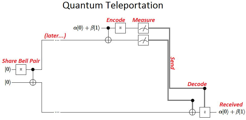
Quantum Teleportation
Alice now has one more qubit, in the state $\alpha |0\rangle + \beta |1\rangle$ She wants to send her qubit to Bob, by changing the state of Bob's entangled qubit to Alice's extra qubit.
Confusing? Let's try naming the qubits. Alice and Bob have the qubits A and B respectively, which are entangled in the bell state. Alice has another qubit C.
Alice wants to send her qubit to Bob by changing the state of B, to that of C. She wants the state of the qubit B to be $\alpha |0\rangle + \beta |1\rangle$. Alice doesn't know the values of a and b. Also, Bob can't make a measurement in any case as doing so will destroy B's state.
How does Alice do it? Well, she first passes both her qubits through the Reverse Bell circuit. She then measures both of her qubits. She gets one of the following outputs: $|00\rangle,|01\rangle,|10\rangle\ \text{and}\ |11\rangle$, each with probability 1/4. Alice sends these two classical bits to Bob, via any classical means, example, she texts him or calls and tells him. Bob knows that corresponding to her message, there are 4 options, and he takes action accordingly for each.
- He gets the message, from Alice and knows that his qubit(qubit B) changed its state to that of qubit C.
- He gets the message, and knows that his qubit changed its state to and he passes his qubit through X gate to change its state to that of qubit C.
- He gets the message, and knows that his qubit changed its state to and he passes his qubit through Z gate to change its state to that of qubit C.
- He gets the message, and knows that his qubit changed its state to and he passes his qubit through Y gate to change its state to that of qubit C.
We implement the following circuit step by step:
We represent the entangled qubit pair shared between Alice and Bob as "Alices_and_Bobs_entangled_qubits". Whereas, Alice has another separate qubit whose state is prepared at random. We show that random state below:
begin
	Alices_and_Bobs_entangled_qubits = ArrayReg(bit"00") + ArrayReg(bit"11") |> normalize!
	Alicequbit = rand_state(1) #This function creates a qubit with a random state.
	state(Alicequbit)
end
state(Alices_and_Bobs_entangled_qubits)
Encoding part of the circuit which is performed by Alice is shown below:
begin
	teleportationcircuit = chain(3, control(1,2=>X), put(1=>H))
	plot(teleportationcircuit)
end
Joining shared bell pair state with the encoding part to represent the pre-measurement part of the circuit.
Note: The join(qubit1, qubit2.....,qubitn) function is used to join multiple qubits. Remember, the circuit takes the qubits as inputs, in reverse order
begin
	feeding = join(Alices_and_Bobs_entangled_qubits, Alicequbit) |> teleportationcircuit
	state(feeding)
end
begin
    feeding_circ = chain(3,  put(2=>H), control(2,3=>X), control(1,2=>X), put(1=>H))
	plot(feeding_circ)
end
Finally measurement of Alice's qubit is performed by Bob.
Note: The RemoveMeasured() parameter in measure!(), first measures the qubits, then removes the measured qubits from the system of qubits.
begin
    meas_circ = chain(3,  put(2=>H), control(2,3=>X), control(1,2=>X), put(1=>H), Yao.Measure(3; locs=(1,2)))
	plot(meas_circ)
end
Alices_measuredqubits = measure!(RemoveMeasured(), feeding, 1:2)
Depending upon the output of Alice's qubit, Bob then perform decoding as follows:
if(Alices_measuredqubits == bit"00")
	Bobs_qubit = feeding
elseif(Alices_measuredqubits == bit"01")
	Bobs_qubit = feeding |> chain(1, put(1=>Z))
elseif(Alices_measuredqubits == bit"10")
	Bobs_qubit = feeding |> chain(1, put(1=>X))
else
	Bobs_qubit = feeding |> chain(1, put(1=>Y))
end
Is Alice's qubit same as Bob's qubit now? You can see that for yourself!
state(Bobs_qubit)
Comparing them side by side! YAY.
[state(Alicequbit) state(Bobs_qubit)]
Gate Compilation
In principle, the final gates that are executed on a quantum hardware depends upon the type of gates they support. These supporting gates are chosen such that they can approximate any unitary operation to any required degree of accuracy.
Few of the such famous universal set of gates are:
- $\{R_x(\theta), R_y(\theta), R_z(\theta), CNOT\}$ (Populary used in superconducting hardware)
- $\{CNOT, H, T\}$ (Also called Clifford+T set)
In order to run any high-level gate, they are broken down into gates that belong one of such universal gate-set.
Example - Toffolli Gate
We read about the toffoli gate above. Let us now break down into both of these universal gatesets.
let
    plot(chain(3, control((1,2), 3=>X))) #Which translates to if the state of the 1st qubit is |1>, perform X gate to the 2nd qubit or "put" the 2nd qubit through the Z gate.
end
Clifford + T set
let
    plot(chain(3, put(3=>H), control(1,3=>X), put(3=>ConstGate.Tdag), control(2,3=>X), put(3=>ConstGate.T), control(1,3=>X), put(3=>ConstGate.Tdag), control(2,3=>X), put(3=>ConstGate.T), put(2=>ConstGate.T), put(3=>H),  control(1,2=>X), put(1=>ConstGate.T), put(2=>ConstGate.Tdag), control(1,2=>X)))
end
Pauli Rotation + CNOT set
$$ H = R_Y(\pi/2)\ R_Z(\pi)$$$$ T = R_Z(\pi/4) $$$$ T^{\dagger} = R_Z(-\pi/4) $$let
plot(chain(3, put(3=>Rz(π)), put(3=>Ry(π/2)), control(1,3=>X), put(3=>Rz(-π/4)), control(2,3=>X), put(3=>Rz(π/4)), control(1,3=>X), put(3=>Rz(-π/4)), control(2,3=>X), put(3=>Rz(π/4)), put(2=>Rz(π/4)), put(3=>Rz(π)), put(3=>Ry(π/2)), control(1,2=>X), put(1=>Rz(π/4)), put(2=>Rz(-π/4)), control(1,2=>X)))
end